11. Appendix: Built-in Plugins
11.1. Cube Plugins
11.1.1. Utilities
11.1.1.1. Append Cube
Description:
Append one cube to another by either lines, bands, samples, or any spatial combination of lines and samples. To use bands, the datacubes must be the same size spatially (lines and samples). To use the lines or samples option, the datacubes must match the number of lines and samples respectively. The option of any spatial will scramble the line/sample representation in order to make a spatially rectangular datacube. For this option, the number of bands between cubes must match.
Usage:
New Name: New name of output cube.
Append Dir: Direction to append cube (lines, bands, samples, or any spatial).
Append Cube: Cube to append.
Outputs:
Appended datacube.
11.1.1.2. Average Channels
Description:
Averages adjacent bands, samples, and/or lines.
Usage:
Spectral, Sample, and Line Averaging: Select the number of adjacent bands (spectral), sample and/or lines to average together.
Return floating points: Option to return floating point values. Otherwise, the data type of input cube is returned.
Outputs:
Datacube with adjacent bands, samples and/or lines averaged.
11.1.1.3. Bad Band Removal
Description:
Remove selected bands from a datacube and optionally interpolate replacements.
Usage:
Start band: First band to remove.
End band: Last band to remove.
Interpolate: If checked, the removed bands will be linearly interpolated from the adjacent bands.
Outputs:
Datacube with the selected bands removed or interpolated.
11.1.1.4. Band Summary Statistics
Description:
Calculates the following summary statistics for a band of data:
minimum value
maximum value
25th, 50th (median), and 75th percentile values
mean
standard deviation
variance
skew
kurtosis
Usage:
Mode: Choose to view by wavelength, band number, or band name, if available.
Wavelength/Band/Band Name selector: Choose wavelength/band to view.
Ignore Zeros: Check this box to exclude any pixel with the value 0 from calculation.
Output Decimal Places: Select the number of decimal places to display for calculated statistics.
Generate Histogram Image: Click this button to plot the distribution of values for the currently selected band.
Outputs:
A single band datacube containing the band summarized.
11.1.1.5. Bin Channels
Description:
Bins (sums) adjacent bands, samples, and/or lines.
Usage:
Spectral, Sample, and Line Binning: Select the number of adjacent bands (spectral), sample and/or lines to bin together. This is a summation, not an average.
Return floating points: Option to return floating point values. Otherwise, the data type of input cube is returned.
Outputs:
Datacube with adjacent bands, samples and/or lines binned.
11.1.1.6. Convert to BIP, BIL or BSQ
Description:
Converts one datacube interleave to another.
Usage:
Input format: Shows current interleave.
Output format: Select desired output interleave.
Outputs:
Datacube rotated to the desired interleave.
11.1.1.7. Count Pixel Values
Description:
Counts unique class labels, maximum pixel probabilities, or minimum spectral angles in a datacube and displays the counts.
Usage:
Apply to a classified cube class labels, classification probabilities, or spectral angles. The tool will compute the number of class label counts, maximum probability counts, or minimum spectral angle counts.
- Input Cube Type: Select Probability, Class Label, or Spectral Angle depending on the input datacube
type.
Band Number: For Class Label cubes, select the band the pixel counts are desired for.
Outputs:
Launches a dialog box containing the counts.
11.1.1.8. Crop Spatially
Description:
Crop a datacube spatially by starting and ending samples and lines.
Usage:
Start Sample: First sample to keep in resulting datacube.
End Sample: Last sample to keep in resulting datacube.
Start Line: First line to keep in resulting datacube.
End Line: Last line to keep in resulting datacube.
Outputs:
Cropped datacube.
11.1.1.9. Crop Wavelengths
Description:
Crops beginning and/or ending bands from datacube by wavelength.
Usage:
Min Wavelength: Starting wavelength of new cube.
Max Wavelength: Ending wavelength of new cube.
Outputs:
Datacube with beginning and/or ending bands cropped.
11.1.1.10. Crop Wavelengths by Band Number
Description:
Crops beginning and/or ending bands from datacube, with bands specified by band number.
Usage:
Min Band: Starting band of new cube.
Max Band: Ending band of new cube.
Outputs:
Datacube with beginning and/or ending bands cropped.
11.1.1.11. Normalize Datacube
Description:
Normalize each pixel (point spectrum) in a datacube.
Usage:
Method:
Unit: Divide each brightness value within a pixel by the sum of all bands in that pixel, such that the sum of brightness across all bands in the pixel after normalization is 1.
Root Mean Square: Divide each brightness value within a pixel by that pixel’s root mean square brightness.
Maximum: Divide each brightness value within a pixel by the maximum that occurs in that pixel, such that the band that contained the maximum value now contains 1 and all other bands contain a number between 0 and 1.
Min-Max: Scales each brightness value within a pixel by subtracting the minimum value that occurs in the pixel and dividing by the maximum, such that the new minimum and maximum values are 0 and 1.
Outputs:
Normalized datacube.
11.1.1.12. Savitzky-Golay Smoothing
Description:
The Savitzky-Golay filter fits data with successive low-degree polynomials using linear least squares, resulting in smoothed data while preserving much of the original signal’s structure. This implementation will optionally return the n-th derivative of the smoothed signal.
Usage:
Number of points: Size of sliding window for polynomial fitting.
Polynomial Degree: Degree of polynomial used to fit.
Differential order: Order of derivative to return.
Outputs:
Smoothed datacube or n-th derivative of smoothed datacube.
References:
11.1.1.13. Scale To One Utility
Description:
Rescales a datacube to 1 by using either the cube’s Reflectance Scale Factor, Ceiling, Bit Depth, of user entered factor.
Usage:
Reflectance Scale Factor: The scaling factor to divide data by. It suggests the value of the cube’s Reflectance Scale Factor, Ceiling, and Bit Depth metavalues, if present and in that order.
Outputs:
Datacube scaled to 1.
11.1.1.14. Spectrally Interpolate Linear Cube
Description:
Spectrally interpolates a datacube to the bands that would have been produced by a linearly calibrated imager with a different slope and intercept. This may be useful for using data from different spectral imagers in a single model or other classification routine.
Usage:
Slope: Enter new slope.
Intercept: Enter new intercept.
Slope multiplier: Set this to 2 for Pika IIi imagers using cameras in format 7 mode 2 or other values to appropriately compensate for on-camera binning.
New band count: Number of output bands desired.
Extrapolate linearly outside original cube waves: Extrapolate linearly if desired cube falls outside of existing data. An error will occur if this condition is true but the option left unchecked.
Outputs:
Datacube interpolated to new wavelengths.
11.1.1.15. Spectrally Resample Cube
Description:
Resamples (interpolates) a datacube to match the wavelengths of a selected text or header file.
Usage:
This tool will prompt the user to select a text file (txt or csv) or a header file (hdr) containing the desired wavelengths. If txt or csv is chosen, the wavelength values should be in the first column in units of nanometers.
Outputs:
Resampled datacube.
11.1.1.16. Spectrally Resample Spectrum to Datacube
Description:
Resamples (interpolates) a Spectrum to match the wavelengths of source datacube.
Usage:
Spectrum: Select the Spectrum to resample.
Outputs:
Resampled Spectrum.
11.1.1.17. Subset Cube Bands
Description:
Build a cube consisting of a subset of the bands of the source cube.
Usage:
3 Band RGB: Preset to return a 3 band cube using default Red, Green, and Blue bands.
3 Band Color IR: Preset to return a 3 band cube using default Infrared, Red, and Green bands.
Bands: If not using the above presets, select the number and wavelengths of each band to return.
Outputs:
Datacube containing the selected subset of bands.
11.1.1.18. Subtract Cube
Description
Subtract one datacube from another, pixel-by pixel and band-by-band. The datacubes must have matching shape (line, band, and sample count).
Usage:
Second Cube: The cube to be subtracted.
Outputs:
A new datacube in which each pixel represents the difference between the source datacube and Second Cube.
11.1.1.19. Subtract Spectrum
Description:
Subtracts a background spectrum from a datacube. This could be a noise or background fluorescence spectrum, for example.
Usage:
Subtract by: Select the Spectrum to subtract.
Return floating points: Option to return a floating point cube. Otherwise, the original cube’s data type is used.
Outputs:
Datacube with spectrum subtracted.
11.1.1.20. Unit Conversion Utility
Description:
Convert a cube’s intensity values by multiplying each element by a constant scale factor.
Usage:
Scale Factor: Number to multiply datacube by.
Return Floating Point: If selected, the cube will be converted to a 32 bit float. Otherwise, the original datatype will be maintained.
11.1.2. Classify
11.1.2.1. Auto Classifier
Description:
This tool incorporates many proven processes of hyperspectral image classification into a easy-to-use pipeline, while minimizing decisions that must be made by the user. It includes: 1. Feature engineering by concatenation of 1st derivatives to Savitsky-Golay smoothed spectra. 2. Dimensionality reduction with Principal Component Analysis 3. Random Forest classifier
Usage:
Classes: Classes are the discrete training datacubes used to build the predictive model. Enter the number of Classes to be used for training, and that number will be reflected in the number of Class datacube selectors below.
Class Number: For each Class number, select the datacube associated with the class.
Outputs:
- A floating point datacube, with each band containing the probability (0-1) of a pixel
belonging that Class, ordered by Class Number.
References:
11.1.2.2. Binary Encoding
Description:
Binary encoding is a simple classification method with a small computational load. Each band within an input spectrum is encoded into zeros and ones depending on whether the band is above or below the spectral mean. An additional encoding is created, using a zero or one to represent whether the first derivative of that band is negative or positive. This encoding is concatenated with the first. The datacube is encoded in the same way. An exclusive or is then used to compare the datacube’s encoding with the input spectrum’s encoding, and the result summed. This provides a single number that provides a measure of similarity between the input spectrum and individual pixels of a datacube.
Usage:
Layers: Select the number of input spectra to classify the datacube against.
Spectrum: Select the input spectrum used for classification.
Outputs:
- A datacube with each band containing the distance of a pixel from a Spectrum,
ordered by input position.
References:
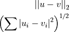
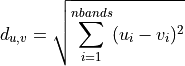
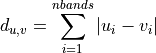
11.1.2.3. Euclidean Distance
Description:
Computes the ordinary straight-line distance in Euclidean space.
where u and v are input vectors (spectra).
Usage:
Layers: Select the number of input spectra to classify the datacube against.
Spectrum: Select the input spectrum used for classification.
Outputs:
- A datacube with each band containing the Euclidean distance of a pixel from a Spectrum,
ordered by input position.
References:
11.1.2.4. Linear Discriminant
Description:
A generalization of Fisher’s linear discriminant that finds a linear combination of features that separate two or more classes, as defined by input training datacubes. It assumes that the independent variables (bands) are normally distributed. It is closely related to logistic regression, which does not make this assumption.
Usage:
Classes: Classes are the discrete training datacubes used to build the predictive model. Enter the number of Classes to be used for training, and that number will be reflected in the number of Class groupings at the bottom of the dialog box. For each Class grouping, select the datacube in the Class field and the associated dependent value in the Group Number field.
Solver: One of either Singular Value Decomposition (svd), Least Squares (lsqr), or Eigenvalue decomposition (eigen). See references below for more information.
N components: Number of components to keep after dimensionality reduction. Must be less or equal to the smaller value between the number of classes minus one, and the number of spectral bands.
Probability: Check to return a probability of class membership, uncheck to return binary predictions.
Tolerance: Threshold for determining whether a singular value is significant. Only used in Singular Value Decomposition.
Outputs:
Datacube with each band containing a probability of a pixel being a member of that class, or a single band with integer encoding that represents class membership by input position order.
References:
11.1.2.5. Logistic Regression
Description:
Logistic regression is a statistical model that uses a logistic function to model a binary dependent variable, in this case membership of a class. Despite the name, it is a linear classification algorithm, not a true regression. It is generally fast and powerful.
Usage:
Reg. Method: Regularization method or penalty. See references for more information.
Probability: Check to return a probability of class membership, uncheck to return integer values indicating the predicted class.
Auto Weight?: Check to automatically adjust training weights to be inversely proportional to class frequencies in the input data. If this option is not checked, the classifier may be more likely to assign pixels to classes that occur more frequently in the training data.
C: Inverse of regularization strength; smaller values specify stronger regularization.
Save coefficients to file: Check to save model coefficients to file for use with other software packages.
Classes: Classes are the discrete training datacubes used to build the predictive model. Enter the number of Classes to be used for training, and that number will be reflected in the number of Class groupings at the bottom of the dialog box. For each Class grouping, select the datacube in the Class field and the associated dependent value in the Group Number field.
Outputs:
Datacube with each band containing a probability of a pixel being a member of that class, or a single band with integer encoding that represents class membership by input position order.
References:
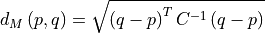
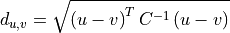
11.1.2.6. Mahalanobis Distance
Description:
Mahalanobis distance quantifies the multivariate similarity between each pixel in a datacube and a distribution defined by all of the pixels in a training datacube (or cubes). The distance used is normalized by the inverse of the covariance matrix computed from the training cubes to adjust for correlations between bands and differences in the magnitude of variance across bands.
Where p is the spectrum at the point being evaluated, q is the mean spectrum computed from the input training cube, and C is the covariance matrix computed from the input training cube. For uncorrelated variables with distributions of equal variance, this reduces to the Euclidean distance.
By applying a threshold to the computed Mahalanobis distance, pixels can be classified as members or outliers of a class.
Usage:
Classes: Classes are the discrete training datacubes used to build the predictive model. Enter the number of Classes to be used for training, and that number will be reflected in the number of Class entries at the bottom of the dialog box. Select Class datacubes for each class.
Outputs:
Datacube with each band containing the Mahalanobis distance between a pixel and the distribution defined by an input class, as ordered by Class datacube input position. Small numbers indicate greater similarity.
References:
11.1.2.7. PLS-DA
Description:
Partial least squares-discriminant analysis is a statistical model that first encodes categorical response variables to a one-hot binary representation, then uses a partial-least squares(PLS) regression to predict the probability of each class membership. PLS regression is a powerful technique for hyperspectral analysis because it uses a cross-decomposition to reduce dimensionality and transform both the response variable (the class membership probabilities) and the input data (the spectral response) to best model the fundamental relationship between the two.
Usage:
Number of Components To Keep: Used by Partial Least Squares as the number of components to use after features have been transformed. With too few components, predictive power may be lost. With too many, the model may be prone to overfitting.
Return Scores?: Check to return a a score proportional to the predicted likelihood of each class membership, with one band per class. Higher values indicate higher likelihood of class membership. Note that these are not probabilities, and may be negative. Uncheck to return integer values indicating the predicted class.
Classes: Classes are the discrete training datacubes used to build the predictive model. Enter the number of Classes to be used for training, and that number will be reflected in the number of Class groupings at the bottom of the dialog box. For each Class grouping, select the datacube in the Class field and the associated dependent value in the Group Number field.
11.1.2.8. Quadratic Discriminant
Description:
Quadratic discriminant analysis is closely related to linear discriminant analysis, but it does not assume the covariance of each of the classes is identical. As a result, it tends to fit data better but has more parameters to estimate.
Usage:
Classes: Classes are the discrete training datacubes used to build the predictive model. Enter the number of Classes to be used for training, and that number will be reflected in the number of Class groupings at the bottom of the dialog box. For each Class grouping, select the datacube in the Class field and the associated dependent value in the Group Number field.
Probability: Check to return a probability of class membership, uncheck to return binary predictions.
Regularization: Parameter to regularize the covariance estimate.
Outputs:
Datacube with each band containing a probability of a pixel being a member of that class, or a single band with integer encoding that represents class membership by input position order.
References:
11.1.2.9. Random Forest
Description:
Random Forest classification is an ensemble method constructed of a multitude of decision trees, each constructed from a random subset of training data and input features. The final output class is the mode of the classes of the individual trees, which helps correct for individual decision trees’ tendency to overfit the training set.
Usage:
Probability: Check to return a probability of class membership (one band for each class), uncheck to return integer class membership predictions as a single band.
Estimators: The number of trees in the forest. Higher numbers tend to produce better predictive models, but require more memory and computational time.
Classes: Classes are the discrete training datacubes used to build the predictive model. Enter the number of Classes to be used for training, and that number will be reflected in the number of Class groupings at the bottom of the dialog box. For each Class grouping, select the datacube in the Class field and the associated dependent value in the Group Number field.
Outputs:
Datacube with each band containing a probability of a pixel being a member of that class, or a single band with integer encoding that represents class membership by input position order.
References:
11.1.2.10. Spectral Angle Mapper
Description:
Compares spectra in a datacube to reference (input) spectra by computing the spectral angle between them. By treating the spectra as vectors, the angle between them is simply the inverse cosine of the normalized dot product of the two.
Thus, two parallel vectors have a spectral angle of zero, while orthogonal vectors have a spectral angle of π/2. These angles are typically thresholded to determine class membership.
Usage:
Layers: Select the number of input spectra to classify the datacube against.
Spectrum: Select the input spectrum used for classification.
Outputs:
Datacube with each band containing the spectral angle between input pixels and reference spectra in radians, ordered by input position of spectrum. Smaller numbers indicate greater similarity.
References:
11.1.2.11. Spectral Unmix
Description:
Assuming that a signal at a given pixel is a linear combination of pure endmember spectra, this tool will return the relative abundances of the input endmember, constrained to a defined range. Useful for both fluorescence and remote sensing data.
Usage:
Constrain To: Constrain the output to the defined range.
Endmembers: Number of input endmember spectra. Select individual endmember spectra in the dropdown boxes.
Outputs:
A datacube with each band containing the relative abundance of the endmember, ordered by input position order.
References:
11.1.2.12. Support Vector Machine
Description:
A SVM model is a representation of the training examples as points in space, mapped so that the examples of the separate categories are divided by a clear gap that is as wide as possible. New examples are then mapped into that same space and predicted to belong to a category based on the side of the gap on which they fall. In addition to performing linear classification, SVMs can efficiently perform a non-linear classification using what is called the kernel trick, implicitly mapping their inputs into high-dimensional feature spaces.
Usage:
Method: One of Linear, Poly, RBF, or LinearSVC, plus the option of returning probability (“Proba”) instead of discrete class predictions. Linear, Poly, or RBF specify the kernel function to use in SVC, wile LinearSVC is very similar to Linear but scales better to large number of samples.
Auto Gamma?: Kernel coefficient for RBF and Polynomial functions.
Auto Weight?: Check to automatically adjust weight inversely proportional to class frequencies in the input data.
C: Inverse of regularization strength; smaller values specify stronger regularization.
Poly Degree: Degree of polynomial kernel function. Not used in other methods.
Classes: Classes are the discrete training datacubes used to build the predictive model. Enter the number of Classes to be used for training, and that number will be reflected in the number of Class groupings at the bottom of the dialog box. For each Class grouping, select the datacube in the Class field and the associated dependent value in the Group Number field.
Outputs:
Datacube with each band containing a probability of a pixel being a member of that class, or a single band with integer encoding that represents class membership by input position order.
References:
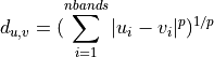
11.1.2.13. k-Nearest Neighbors
Description:
Neighbors-based classification is computed from a simple majority vote of the nearest neighbors of each point based on a distance metric. To avoid prohibitively long computation times, it is recommended to reduce dimensionality before using k-NN.
Usage:
N Neighbors: Number of neighbors to use in vote.
Weights: Select uniform to have all points in neighborhood weighted equally. Select distance to weight by inverse distance.
Distance Metric: Distance metric used to compute similarity of neighbors.
- euclidean - ordinary straight line distance in n-dimensional space
- manhattan - the sum of the absolute differences in each dimension in n-dimensional space
- mahalanobis - a statistically weighted distance that accounts for correlations and scale
- differences between bands.
where u and v are the point vectors being compared and C is the covariance matrix computed from the complete dataset.
- minkowski - a generalization of euclidean and manhattan distance defined as
Setting P to 1 is equivalent to Manhattan distance, P = 2 is equivalent to Euclidean.
- chebyshev - the maximum distance in a single dimension between two point vectors
See references for more information.
Power (P): Power to be used in the Minkowski distance calculation. Setting P to 1 is equivalent to Manhattan distance, P = 2 is equivalent to Euclidean.
Probability: Check to return a probability of class membership, uncheck to return discrete predictions.
Classes: Classes are the discrete training datacubes used to build the predictive model. Enter the number of Classes to be used for training, and that number will be reflected in the number of Class groupings below. For each Class grouping, select the datacube in the Class field and the associated dependent value in the Value field.
Outputs:
Datacube with each band containing a probability of a pixel being a member of that class, or a single band with integer encoding that represents class membership by input position order.
References:

11.1.3. Analyze
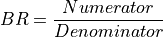
11.1.3.1. Band Ratio
Description:
Divide each pixel in one band by those in another band.
Usage:
Numerator Wavelength: The wavelength of the band in the numerator of the ratio.
Denominator Wavelength: The wavelength of the band in the denominator of the ratio.
Outputs:
A new single band floating point datacube from the ratio.
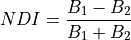
11.1.3.2. Custom Normalized Difference Index
Description:
Calculate a custom normalized difference index for each pixel, defined as:
If the denominator is zero for any pixels, the return value of those pixels will be set to zero.
Usage:
First Band: The wavelength of the first band.
Second Band: The wavelength of the second band.
Outputs:
A floating point cube of the normalized difference.
11.1.3.3. First Derivative
Description:
Compute the first derivative along the spectral axis.
Usage:
Smoothed implementation: If true, the derivative is calculated using a Savitzky-Golay filter (recommended). If False, a simple band-to band difference is used (rise / run). This tends to produce noisy results. For fine grained control over the parameters of smoothing used, use the Savitzky-Golay Smoothing plugin instead of this version.
Outputs:
A floating point datacube of the first derivative.
11.1.3.4. Matched Filter
Description: The matched filter is designed to detect the presence of and contribution of a known signal (target spectrum) within each pixel of a datacube.
Usage:
Target spectrum: The signal to detect.
Background cube: a cube that represents the typical background environment of the target area. By default, the plugin uses the currently loaded datacube as the background.
Outputs: A scalar indicating the strength of the match between the target and each pixel in the datacube. Higher values indicate greater contribution of the target spectrum.
11.1.3.5. Minimum Noise Fraction
Description:
The Minimum Noise Fraction is a linear transformation of two separate principal component analysis (PCA) rotations. The first rotation utilizes the principal components of the noise covariance matrix to ensure the noise has unit variance and are spectrally uncorrelated. The second PCA rotation is applied to the original data after it has been noise whitened by the first.
Usage:
Bands To Return: The number of rotated bands to retain after the transformation.
Standardize: If this is checked, data is normalized band-wise prior to the transformation by subtracting the mean and dividing by the standard deviation. Unless the input datacube has already been standardized, this should usually be set to True because PCA is sensitive to scale variations across bands.
Est. Noise from Dark Field: If checked, the user will be prompted for a dark noise cube to estimate noise from. If unchecked, the noise will be estimated from the input data.
Outputs:
A new floating point cube containing the MNF scores of the transformed data.
The scree plot of eigenvalues is plotted in the User Plot window.
References:
1. Green, A.A., M. Berman, p. Switzer and M.D. Craig (1988) A transformation for ordering multispectral data in terms of image quality with implications for noise removal. IEEE Transactions on Geoscience and Rmote Sensing, 26(1):65-74.
11.1.3.6. PCA
Description:
Principal Component Analysis is an orthogonal linear transformation of data such that the new coordinate system orders bands by decreasing magnitude of explained total variance. The transformation is determined by the eigen decomposition of the covariance matrix. Typically, a relatively small subset of the resulting bands are retained after the coordinate rotation to reduce the dimensionality of the dataset.
Usage:
Bands To Return: The number of rotated bands to retain after the transformation.
Standardize: If this is checked, data is normalized bandwise prior to the transformation by subtracting the mean and dividing by the standard deviation. Unless the input datacube has already been standardized, this should usually be set to True because PCA is sensitive to scale variations across bands.
Save Transformation Matrix: If this is checked, a transformation matrix is saved to disk, which can can be used to apply the same transformation to other cubes using the PCA from Prior Transform plugin.
Outputs:
A new floating point cube containing the PCA scores of the transformed data.
The scree plot of eigenvalues is plotted in the User Plot window.
References:
11.1.3.7. PCA from Prior Transform
Description:
Uses a previously saved PCA transformation (from the PCA plugin) to transform other data.
Usage:
Bands To Return: The number of rotated bands to retain after the transformation.
Standardize: If this is checked, data is normalized bandwise prior to the transformation by subtracting the mean and dividing by the standard deviation of the data used to originally fit the transform. Unless the input datacube has already been standardized, this should usually be set to True because PCA is sensitive to scale variations across bands.
PCA Transformation Matrix: Once OK has been pressed, the software will prompt for the previously saved transform.
Outputs:
A new floating point cube containing the PCA scores of the transformed data.
The scree plot of eigenvalues is plotted in the User Plot window.
References:
11.1.3.8. Regression
Description:
A collection of different statistical methods for predicting a dependent variable (or outcome variable), from one or more independent variables, typically bands in the context of hyperspectral imaging.
Usage:
Method: Can be one of Support Vector (Linear), Support Vector (Radial Basis Function), Ordinary Least Squares, Partial Least Squares, Lasso, Ridge, Ridge (with Cross Validation). Partial Least Squares is a good place to start. See references for more information on these methods.
Alpha: This parameter is used in Ridge and Lasso as the regularization strength parameter. Larger values increase regularization and reduce variance of the estimate.
Auto Gamma: Uncheck this box to specify gamma manually.
Gamma: This parameter is used in SVR RBF to set how far the influence of a single training example reaches, low values meaning greater influence. It can be thought of as the inverse of the radius of influence of model-selected support vectors.
Penalty: This parameter is the regularization parameter, C, used by SVR. The strength of the regularization is inversely proportional to C.
Fit Intercept: Used in OLS, Lasso, Ridge, and RidgeCV to determine whether to calculate the intercept. If data has already been centered, fitting an intercept is not necessary.
Number of Components To Keep: Used by Partial Least Squares as the number of components to use after features have been transformed. With too few components, predictive power may be lost. With too many, the model may be prone to overfitting.
Classes:
Classes are the discrete training datacubes used to build the predictive model. Enter the number of Classes to be used for training, and that number will be reflected in the number of Class groupings below. For each Class grouping, select the datacube in the Class field and the associated dependent value in the Value field.
Outputs:
A floating point datacube containing the predicted dependent variable.
References:
11.1.3.9. Second Derivative
Description:
Compute the second derivative along the spectral axis.
Usage:
Smoothed implementation: If true, the derivative is calculated using a Savitzky-Golay filter (recommended). If False, a simple band-to band difference is used (rise / run). This tends to produce noisy results. For fine grained control over the parameters of smoothing used, use the Savitzky-Golay Smoothing plugin instead of this version.
Outputs:
A floating point datacube of the second derivative.
11.1.3.10. Thinfilm Thickness
Description:
This algorithm finds the distance between peaks of interference spectra and uses this distance, along with the known Index of Refraction and angle of incidence, to compute film thickness in microns. The sample must be clean and have a mirror finish.
Usage:
Angle of Incidence: Angle between incident light and normal. Imager should be setup at the same angle on the other side of normal.
Index of Refraction: Measured or previously determined IOR of film.
Show Advanced Settings? Show smoothing and peaking finding settings.
SavGol Window Length: Length of Savistky-Golay smoothing window.
SavGol Order: Polynomial order of Savistky-Golay smoothing.
Peak Prominence: Threshold of peak prominence of peak. Lower numbers are more inclusive.
Show Example Fit? Check to see example of peak finding solution and the below line, sample.
Example Line Number: Line number of example peak finding plot.
Example Sample Number: Sample number of example peak finding plot.
Outputs:
A floating point datacube of the film thickness in microns.
References:
11.1.3.11. Total Radiance
Description:
Sums all bands of a datacube in units of radiance to produce total radiance. May also be used to sum any band data into a single band datacube.
Outputs:
A single band floating point datacube.
11.1.4. Correct
11.1.4.1. Back Out Raw Data from Reflectivity
Description:
Convert reflectance data back to raw data from a datacube containing the original white reference and optional dark current datacube.
Usage:
The input datacube must be in units of reflectance.
100% Reflectivity Scaled To: The scaling of the input reflectance datacube.
Correction Cube: The white reference datacube used to originally convert the data to reflectance.
Dark Noise Cube: The optional dark noise datacube used to originally covert data to reflectance.
Outputs:
A datacube of uncorrected (raw) data.
11.1.4.2. Correct Optical Distortion
Description:
A Brown-Conrady radial distortion model in the across track dimension to correct for distortions. No tangential distortion coefficients used in this model.
Usage:
K1 through K4: These are the radial distortion coefficients. Contact the objective lens manufacturer or Resonon to obtain these coefficients.
Outputs:
A corrected datacube.
References:
http://en.wikipedia.org/wiki/Distortion_(optics)#Software_correction
11.1.4.3. Georectify Airborne Datacube (not installed)
Description:
Creates georectified output products based on GPS/IMU data.
Usage:
Use Flat Earth Elevation: Check to use flat earth elevation below, uncheck to use DEM file.
Flat Earth Elev. (m): The elevation of the ground in the area the datacube was collected.
Field of View (deg): The field of view of the imager/lens combination used.
Calculated Resolution (m): An estimate of the cross and along track resolutions using the FOV and average above ground height for cross track, and distance flown and frame rate for along track. The recommended resolution is twice the largest estimate, to account for platform instabilities.
Map Resolution (m): Desired resolution of output products, in meters.
Override heading with course? Overrides the heading with GPS course. This may be useful for poor heading accuracy datasets if the system is well aligned with the direction of aircraft flight.
Save Products in Source Folder?: Check to save all products (beside Full Datacube) in original folder. Uncheck to specify destination.
Generate Full Datacube?: Creates a georectified datacube and adds it to the Resource Tree in Spectronon. It is not saved automatically like the other output products.
Generate KML of Image?: Check to generate a KML file of the selected Image.
Generate GeoTiff of Image?: Check to generate a GeoTiff of the selected Image.
Generate Swath Outline?: Check to generate an outline of the FOV down the flight path, useful for debugging.
Interpolate Image?: If checked, the missing pixels of the GeoTiff/KML images will be interpolated.
Interpolate Datacube?: If checked, the missing pixels of the datacube will be interpolated.
Average Overlapping Pixels?: If checked, pixels with multiple projections will contain the average of all projected spectra. Otherwise the pixel will contain the spectrum of the last projection. Does not apply to images, only full datacubes.
Image To Use in KML/GeoTiff: Select which Image to use in KML/GeoTiff (order follows Resource Tree)
Stretch: Apply the specified stretch to GeoTiff/KML image. Absolute is recommended.
Low/High: Absolute stretch values.
Sync Offset (s): Time delay between image data and GPS/IMU.
Imager Roll Offset (deg): Angular offset in the roll direction between imager nadir and IMU nadir.
Imager Pitch Offset (deg): Angular offset in the pitch direction between imager nadir and IMU nadir.
Imager Heading Offset (deg): Angular offset between imager and IMU in the heading direction.
Crop Cube to Start/End Lines?: Used to crop beginning and or ending of datacube in the geocorrection process.
Outputs:
All outputs are optional.
KML and GeoTiff of Image.
A georectified datacube.
Outline KML of imager FOV along flight path.
Mask of interpolated pixels
Interpolated LCF file
References:
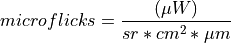
11.1.4.4. Radiance From Raw Data
Description:
Converts raw data to units of radiance (microflicks) based on the instrument’s radiometric calibration file (.icp). This process is outlined below:
The .icp file contains multiple calibration files, one gain cube that contains the pixel-by-pixel transfer from digital number to calibrated radiance and typically many offset cubes, which are dark noise cubes taken at different integration times and gains. This plugin automatically finds the best suited offset file to use (Auto Remove Dark) unless the user decides to provide one.
The gain and offset files are scaled to match the binning factor used in the datacube. Note that because the gain file represents the inverse instrument response, it gets scaled inversely.
The gain and offset data are averaged both spatially and spectrally to match the frame size of the datacube.
The gain and offset data are flipped spatially depending on the flip radiometric calibration header item in the datacube. (This header item is used to track left-right edges in airborne data.)
The gain data is scaled by the integration and gain ratios between it and the datacube. Note that gain in Resonon headers is 20 log, not 10 log.
The offset data is subtracted from the datacube. The result is multiplied by the gain file.
The resulting data is in units of microflicks.
Usage:
The datacube must be collected with a Resonon instrument with a supplied Imager Calibration Pack (.icp).
Auto Remove Dark Noise: Select to use the most appropriate dark noise file in the ICP file. Uncheck for user supplied dark noise datacube.
Return floating point: By default, the result is returned as a two byte integer because solar illuminated scenes in units of radiance will never exceed 2^16 uFlicks. For very bright light sources or very dimly illuminated scenes, floating point numbers are necessary.
Set Saturated Pixels to Zero?: This option will set saturated pixels to zero after the radiance conversion process as it is difficult to detect saturation after radiance conversion otherwise.
Saturation Value: Level at which saturation occurs. Defaults to the ceiling value in the header or the bit depth value if ceiling is not available. User can overide.
Outputs:
A datacube containing calibrated radiance units of microflicks.
References:
11.1.4.5. Raw Data From Radiance
Description:
Converts radiance (microflicks) to units of raw data (DN) based on the instrument’s radiometric calibration file (.icp). It is designed as the inverse of the Radiance From Raw Data plugin. This process is outlined below:
The .icp file contains multiple calibration files, one gain cube that contains the pixel-by-pixel transfer from digital number to calibrated radiance and typically many offset cubes, which are dark noise cubes taken at different integration times and gains. This plugin automatically finds the best suited offset file to use (Auto Remove Dark) unless the user decides to provide one.
The gain and offset files are scaled to match the binning factor used in the datacube. Note that because the gain file represents the inverse instrument response, it gets scaled inversely.
The gain and offset data are averaged both spatially and spectrally to match the frame size of the datacube.
The gain and offset data are flipped spatially depending on the flip radiometric calibration header item in the datacube. (This header item is used to track left-right edges in airborne data.)
The gain data is scaled by the integration and gain ratios between it and the datacube. Note that gain in Resonon headers is 20 log, not 10 log.
The datacube is divided by the gain file. The offset is added to the result.
The datacube is then clipped (np.clip) at 0 and the saturation value to correct for any errors in the inversion process.
The resulting data is in units of digital numbers.
Usage:
The datacube must be collected with a Resonon instrument with a supplied Imager Calibration Pack (.icp).
Undo Auto Remove Dark Noise: Select to use the most appropriate dark noise file in the ICP file. Uncheck for user supplied dark noise datacube. If the image was calibrated to radiance using a supplied dark noise datacube, that same datacube should be used to convert back to raw data.
Outputs:
A datacube containing raw data in digital numbers.
References:
11.1.4.6. Reflectance from Radiance Data and Downwelling Irradiance Spectrum
Description:
Converts radiance data to reflectivity based on a downwelling irradiance spectrum collected with a single point spectrometer and cosine corrector. This approach assumes the surfaced imaged is Lambertian. Reflectance is then found by:
where L is the at-sensor radiance from the imager and E is the downwelling irradiance.
Usage:
Downwelling Type: Choose either Resonon supplied or other vendor calibrated unit.
Use Downwelling Spectrum in Source Folder: Check to automatically use spectrum in same folder as the source code. Uncheck for user supplied downwelling spectrum (open in Spectronon)
Downwelling Calibration: Resonon supplied downwelling calibration file (.dcp)
Auto Remove Downwelling Dark Noise: Check to use previously measured dark noise (inside DCP file). Uncheck for user supplied dark noise spectrum.
Scale 100% Reflectivity To: Scaling factor for output datacube.
Use Correlation Coefficients: Use previously computed Correlation Coefficients to align downwelling data to ground truth.
Outputs:
Datacube containing reflectivity values.
References:

11.1.4.7. Reflectance from Radiance Data and Measured Reference Spectrum
Description:
This approach to converting data to reflectance assumes the input datacube has been corrected spatially, typically by converting to radiance but other approaches would be acceptable. A spectrum of measured reference material is used to correct the datacube spectrally. This spectrum should be collected with the same instrument under the same conditions as the datacube to be collected. The measured reflectance should be a tab, space, or comma delimited file with the first column containing wavelength in nanometers and the second column containing reflectance, scaled to either 0-1 or 0-100%.
Usage:
The input datacube should be in units of radiance (or spatially corrected by other means). The input spectrum is typically created with a region-of-interest tool of reference material in a datacube collected with the same imager and under the same conditions.
Measured Reflectivity: Click this button to select the tab, space, or comma delimited file containing the measured reflectance spectrum of the reference material.
Measured Reflectivity in Percentage?: Check this box if measured reflectivity is scaled to 0-100. If unchecked, a scale of 0-1 is assumed.
ROI Spec: Spectrum of measured reference material.
Scale 100% Reflectivity To: Scaling factor for output datacube.
Outputs:
A floating point datacube of reflectance data, scaled to the selected factor.
11.1.4.8. Reflectance from Radiance Data and Spectrally Flat Reference Spectrum
Description:
This approach assumes the input datacube has been corrected spatially, typically by converting to radiance but other approaches would be acceptable. A spectrum of spectrally flat reference material (typically Spectralon ™ or Fluorilon ™) is used to correct the datacube spectrally. This spectrum should be collected with the same instrument under the same conditions as the datacube to be corrected.
Usage:
The input datacube should be in units of radiance (or spatially corrected by other means). The input spectrum is typically created with a region-of-interest tool of spectrally flat material in a datacube collected with the same imager and under the same conditions.
ROI Spec: Spectrum of spectrally flat reference material.
Flat Reflectivity (0-1): Reflectivity of reference material on a scale of 0-1 (0-100%).
Scale 100% Reflectivity To: Scaling factor for output datacube.
Outputs:
A floating point datacube of reflectance data, scaled to the user’s choice.
11.1.4.9. Reflectance from Raw Data and Downwelling Irradiance Spectrum
Description:
Converts raw data to reflectivity based on a downwelling irradiance spectrum collected with a single point spectrometer and cosine corrector. This approach assumes the surfaced imaged is Lambertian. Reflectance is then found by:
where L is the at-sensor radiance from the imager and E is the downwelling irradiance.
Usage:
Imager Calibration: Resonon supplied imager calibration (.icp) file
Auto Remove Dark Noise: Check to use previously measured dark noise (inside ICP file). Uncheck for user supplied dark noise cube.
Downwelling Type: Choose either Resonon supplied or other vendor calibrated unit.
Use Downwelling Spectrum in Source Folder: Check to automatically use spectrum in same folder as the source code. Uncheck for user supplied downwelling spectrum (open in Spectronon)
Downwelling Calibration: Resonon supplied downwelling calibration file (.dcp)
Auto Remove Downwelling Dark Noise: Check to use previously measured dark noise (inside DCP file). Uncheck for user supplied dark noise spectrum.
Scale Downwelling Dark Noise to Signal Tail: This feature estimates the dark noise of the downwelling sensor at bands with no signal and scales the dark correction to match.
Scale 100% Reflectivity To: Scaling factor for output datacube.
Use Correlation Coefficients: Use previously computed Correlation Coefficients to align downwelling data to ground truth.
Set Saturated Pixels to Zero?: This option will set saturated pixels to zero after the radiance conversion process as it is difficult to detect saturation after radiance conversion otherwise.
Saturation Value: Level at which saturation occurs. Defaults to the ceiling value in the header or the bit depth value if ceiling is not available. User can overide.
Outputs:
Datacube containing reflectivity values.
References:
11.1.4.10. Reflectance from Raw Data and Measured Reference Cube
Description:
Convert raw data to reflectance based on a input datacube of measured reference material. This datacube needs to have the reference material fill the entire FOV of the instrument, and be collected with the same instrument under the same conditions as the datacube to be corrected. The measured reflectance should a tab, space, or comma delimited file with the first column containing wavelength in nanometers and the second column containing reflectance, scaled to either 0-1 or 0-100%.
Usage:
The input datacube should be in units of radiance (or spatially corrected by other means). The input spectrum is typically created with a region-of-interest tool of reference material in a datacube collected with the same imager and under the same conditions.
Measured Reflectivity: Click this button to select the tab, space, or comma delimited file containing the measured reflectance spectrum of the reference material.
Measured Reflectivity in Percentage?: Check this box if measured reflectivity is scaled to 0-100. If unchecked, a scale of 0-1 is assumed.
ROI Spec: Spectrum of measured reference material.
Scale 100% Reflectivity To: Scaling factor for output datacube.
Outputs:
A floating point datacube of reflectance data, scaled to the user’s choice.
11.1.4.11. Reflectance from Raw Data and Spectrally Flat Reference Cube
Description:
Converts raw data to reflectivity based on another datacube of a spectrally flat reference material. This datacube needs to have the reference material fill the entire FOV of the instrument, and be collected with the same instrument under the same conditions as the datacube to be corrected.
Usage:
Correction Cube: Datacube of spectrally flat reference material.
Flat Reflectivity (0-1): Reflectivity of reference material on a scale of 0-1 (0-100%).
Scale 100% Reflectivity To: Scaling factor for output datacube.
Outputs:
A floating point datacube of reflectance data, scaled to the user’s choice.
11.1.4.12. Remove Dark Noise From Cube
Description:
Subtracts a frame of dark noise from a datacube. This frame can be a single frame of data, or a datacube of dark noise. If a datacube is used, its lines are averaged to create a single frame.
Usage:
Dark Noise Cube: Datacube of recorded dark noise.
Outputs:
A datacube with dark noise removed.
11.1.5. Anomaly
11.1.5.1. Elliptic Envelope Anomaly
Description: Anomalies are detected by estimating a robust covariance of the dataset, fitting an ellipse to the central data points, and ignoring those outside. Mahalanobis distances are used to determine a measure of a point’s likelihood of being an outlier.
Usage:
The method assumes a Gaussian distributed dataset. For other distributions, other algorithms may perform better, such as SVM Anomaly with the RBF kernel.
Outlier detection from covariance estimation may break or not perform well in high-dimensional settings. In particular, one will always take care to work with n_samples > n_features ** 2. Feature reduction should be performed prior in order to accelerate run times.
Clutter: Datacube containing only the statistical normal background, without any outliers.
Outputs: Floating point datacube containing +1 for inliers and -1 for outliers.
References:
11.1.5.2. Least Squares Anomaly
Description: Probabilistic method for the detection of anomalous outliers based on a squared-loss function.
Usage:
Clutter: Datacube containing only the statistical normal background, without any outliers.
Probability: If checked, the probability of a pixel being anomalous is returned, scaled 0-1. If unchecked, a classification is returned, with 0 being inliers and 1 for outliers.
Outputs: If Probability is checked, a floating point datacube containing a 0-1 probability is returned. If not, a floating point datacube of 0 for inliers and 1 for outliers is returned.
References:
1. J.A. Quinn, M. Sugiyama. A least-squares approach to anomaly detection in static and sequential data. Pattern Recognition Letters 40:36-40, 2014.
11.1.5.3. RX Anomaly Detector
Description:
The Reed-Xiaoli (RX) anomaly detector detects pixels determined to be spectrally anomalous relative to a user-defined background or neighboring region. It assumes that the background can be modeled by a multivariate Gaussian distribution. The Mahalanobis distance between a given pixel and the background model is calculated and compared to a user-defined threshold, determining whether the pixel belongs to the background or is an anomaly.
Usage:
Global: Compares each pixel to the entire datacube.
Local (Lines): Compares each pixel to the image area within a user-defined number of lines of the pixel under test.
Local (Squares): Compares each pixel to a square image area of the user-defined size adjacent to the pixel under test.
User Selected: Compares each pixel to a user supplied datacube that defines the expected background (also known as clutter).
Outputs:
A floating point datacube containing the Mahalanobis distance to the selected background area. The default Image for this cube is the Threshold To Colormap, which allows the user to threshold the results to better highlight anomalies.
References:
1. Reed I., and X. Yu, “Adaptive Multiple-Band CFAR Detection of an Optical Pattern with Unknown Spectral Distribution.” IEEE Transactions on Acoustics, Speech and Signal Processing 38 (1990): 1760-1770.

11.1.5.4. SVM Anomaly
Description: Anomalies are detected using a One Class Support Vector Machine with a user-supplied background (or clutter) datacube. This cube should contain only statistical normal pixels (without anomalies).
Usage:
As with other Support Vector Machines, feature reduction should be performed prior in order to accelerate run times.
Method: Can be one of Linear, Radial Basis Function (RBF), or Polynomial. See references for more information on these methods.
Clutter: Datacube containing only the statistical normal background, without any outliers.
Nu: Upper bound on the fraction of training errors and a lower bound of the fraction of support vectors.
Auto Gamma: If selected, the gamma kernel coefficient is set to 1/(number of features).
Gamma: Kernel coefficient for RBF and polynomial functions.
Degree: Degree of the polynomial kernel function.
Outputs: Floating point datacube containing +1 for inliers and -1 for outliers.
References:
11.1.6. Color
11.1.6.1. CIE Colorspace Conversion
Description:
The CIE colorspace is a color coordinate system based on the human eye’s response to light and color. It is a mathematical generalization of human color vision, allowing one to define and reproduce colors in a objective way.
Usage:
The input datacube must be in units of reflectance with a reflectance scale factor header item, ideally with a spectral range of 390-700 nm.
Illuminant: The theoretical source of light in order to compare colors across different lighting.
Standard Observer: The observer function is the model of human vision produced from color matching experiments. The response of the eye is a function of the field of view, standard values being 10 and 2 degrees.
XYZ: The CIE XYZ color space is the extrapolation of RGB to avoid negative numbers. The Y parameter is a measure of the luminance, with X and Z specifying the chromaticity, with Z somewhat equal to blue and X is a mix of cone response chosen to be orthogonal to luminance.
xyY: In CIE xyY, Y is the luminance and x and y represents the chrominance values derived from the tristimulus values X, Y and Z in the CIE XYZ color space.
L*a*b:* L*a*b* is a color model and space in which L is brightness and a and b are chrominance components. It contains color values far more than the human gamut, but designed to be device independent.
Outputs:
A floating point datacube containing XYZ, xyY, and/or L*a*b* values.
References:
11.1.6.2. Delta E*
Description:
The distance metric of Delta E* is measure of color difference in L*a*b* space. It is meant that a Delta E* of one is a just noticeable difference across the entire gamut. In practice, a Delta E* of about 2.3 is just noticeable. It is defined as:
Usage:
The input datacube must have L*a*b* bands named L* (L*a*b*), a* (L*a*b*), b* (L*a*b*).
Member Count: The number of L*a*b* values to compute distances to.
L*, a*, b*: Values to find Delta E* distances to.
Outputs:
A floating point datacube containing Delta E* distances to each input L*a*b* value.
References:

11.1.6.3. XYZ to RGB Colorspace Conversion
Description:
Convert CIE XYZ colorspace to a RGB colorspace.
Usage:
The input datacube must have bands containing XYZ data, named X (XYZ), Y (XYZ), and Z (XYZ).
RGB Working Space: Desired RGB space to output.
Companding: The desired non-linear transformation of intensity values.
Result datatype: The desired output datatype and bit-depth.
Outputs:
A floating point datacube containing RGB values.
References:
11.1.7. Agricultural
11.1.7.1. Anthocyanin Reflectance Index 1
Description:
Index sensitive to relative concentrations of anthocyanin versus chlorophyll pigments. As plants are stressed the leaves contain higher concentrations of anthocyanin pigments. New leaves also have high anthocyanin concentrations. Data should be in units of reflectance.
The wavelengths of Green and Red are 550 and 700 nm respectively.
Outputs:
A floating point datacube of CRI data.
References:
Gitelson, A., M. Merzlyak, and O. Chivkunova. “Optical Properties and Nondestructive Estimation of Anthocyanin Content in Plant Leaves.” Photochemistry and Photobiology 71 (2001): 38-45
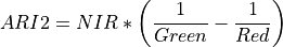
11.1.7.2. Anthocyanin Reflectance Index 2
Description:
Index sensitive to relative concentrations of anthocyanin versus chlorophyll pigments. As plants are stressed the leaves contain higher concentrations of anthocyanin pigments. New leaves also have high anthocyanin concentrations. Data should be in units of reflectance.
The wavelengths of Green, Red, and NIR are 550, 700, and 800 nm respectively.
Outputs:
A floating point datacube of ARI2 data.
References:
Gitelson, A., M. Merzlyak, and O. Chivkunova. “Optical Properties and Nondestructive Estimation of Anthocyanin Content in Plant Leaves.” Photochemistry and Photobiology 71 (2001): 38-45
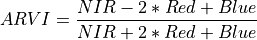
11.1.7.3. Atmospherically Resistant Vegetation Index
Description:
Atmospherically Resistant Vegetation Index robust to atmospheric aerosols and topographic effects.
The wavelengths of the NIR, Red, and Blue bands are 800, 680, and 450 nm respectively.
Outputs:
A floating point datacube of ARVI data.
References:
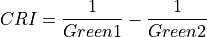
11.1.7.4. Carotenoid Reflectance Index 1
Description:
Index sensitive to carotenoid versus chlorophyll pigments. As plants are stressed the leaves contain higher concentrations of carotenoid pigments. Values for green vegetation range from 1 to 12. Data should be in units of reflectance.
The wavelengths of Green1 and Green2 are 510 and 550 nm respectively.
Outputs:
A floating point datacube of CRI data.
References:
Gitelson, A., M. Merzlyak, and O. Chivkunova. “Optical Properties and Nondestructive Estimation of Anthocyanin Content in Plant Leaves.” Photochemistry and Photobiology 71 (2001): 38-45
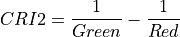
11.1.7.5. Carotenoid Reflectance Index 2
Description:
Index sensitive to carotenoid versus chlorophyll pigments. As plants are stressed the leaves contain higher concentrations of carotenoid pigments. Values for green vegetation range from 1 to 11. Data should be in units of reflectance.
The wavelengths of Green and NIR are 510 and 700 nm respectively.
Outputs:
A floating point datacube of CRI data.
References:
Gitelson, A., M. Merzlyak, and O. Chivkunova. “Optical Properties and Nondestructive Estimation of Anthocyanin Content in Plant Leaves.” Photochemistry and Photobiology 71 (2001): 38-45
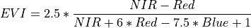
11.1.7.6. Enhanced Vegetation Index
Description:
Enhanced Vegetation Index is optimized for vegetation signal and reduced atmospheric influence.
The wavelengths of the NIR, Red, and Blue bands are 800, 680, and 450 nm respectively.
Outputs:
A floating point datacube of EVI data.
References:
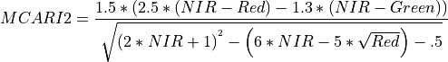
11.1.7.7. Modified Chlorophyll Absorption Ratio Index Improved (MCARI2)
Description:
Index sensitive to the relative abundance of chlorophyll. An improvement of MCARI for better prediction of Leaf Area Index.
The wavelengths of Green, Red, and NIR are 550, 670 and 800 nm respectively.
Outputs:
A floating point datacube of MCARI2 data.
References:
Haboudane, D., et al. “Hyperspectral Vegetation Indices and Novel Algorithms for Predicting Green LAI of Crop Canopies: Modeling and Validation in the Context of Precision Agriculture.” Remote Sensing of Environment 90 (2004): 337-352.
11.1.7.8. Modified Chlorophyll Absorption Reflectance Index
Description:
Index sensitive to the relative abundance of chlorophyll.
The wavelengths of Green, Red, and NIR are 550, 670 and 700 nm respectively.
Outputs:
A floating point datacube of MCARI data.
References:
Daughtry, C., et al. “Estimating Corn Leaf Chlorophyll Concentration from Leaf and Canopy Reflectance.” Remote Sensing Environment 74 (2000): 229-239.

11.1.7.9. Modified Red Edge Normalized Vegetation Index
Description:
Narrowband vegetation index robust to leaf specular reflections.
The wavelengths of the NIR, Red, and Blue bands are 750, 705, and 445 nm respectively. Vegetation has values typically between .2 and .7.
Outputs:
A floating point datacube of MRESRI data.
References:
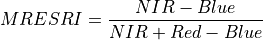
11.1.7.10. Modified Red Edge Simple Ratio Index
Description:
Narrowband vegetation index robust to leaf specular reflections.
The wavelengths of the NIR, Red, and Blue bands are 750, 705, and 445 nm respectively. Vegetation has values typically between 2 and 8.
Outputs:
A floating point datacube of MRESRI data.
References:
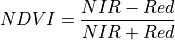
11.1.7.11. Normalized Difference Vegetation Index (NDVI)
Description:
NDVI is an indicator of live green vegetation, primarily qualitatively but also useful as a quantitative tool. It serves as an estimate of the contrast of the red-edge feature of chlorophyll. It is defined as:
The wavelengths of the NIR and Red bands are 800 and 680 nm respectively. NDVI returns a value between -1 and 1. Green vegetation is typically between .2 and .8.
Outputs:
A floating point datacube of NDVI data ranging between -1 and 1.
References: 1. https://en.wikipedia.org/wiki/Normalized_difference_vegetation_index
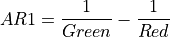
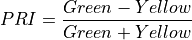
11.1.7.12. Photochemical Reflectance Index
Description:
Vegetation index sensitive to carotenoid pigments in live foliage.
The wavelengths of the Green and Yellow are 570 and 531 nm respectively.
Outputs:
A floating point datacube of PRI data.
References:
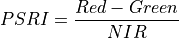
11.1.7.13. Plant Senescence Reflectance Index
Description:
Plant Senescence index sensitive to ratio of carotenoid pigments to chlorophyll.
The wavelengths of the NIR, Green and Red are 750, 500 and 680 nm respectively.
Outputs:
A floating point datacube of PSRI data.
References:
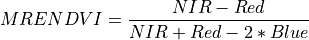
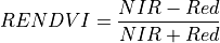
11.1.7.14. Red Edge Normalized Difference Vegetation Index
Description:
Similar to NDVI but using the middle of the Red Edge for the red band.
The wavelengths of the NIR and Red bands are 750 and 705 nm respectively. NDVI returns a value between -1 and 1. Green vegetation is typically between .2 and .9.
Outputs:
A floating point datacube of RENDVI data.
References:
11.1.7.15. Simple Ratio Index
Description:
Simple Ratio is a quick way to distinguish green plants from a background. It is defined as:
The wavelengths of the NIR and Red bands are 850 and 675 nm respectively. Green vegetation has a resulting ratio much greater than one and most other objects close to one.
Outputs:
A floating point datacube of SR data.
References:

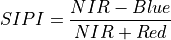
11.1.7.16. Structure Insensitive Pigment Index
Description:
Vegetation index sensitive to carotenoid pigments while minimizing impact of canopy structure.
The wavelengths of the NIR, Blue and Red are 800, 445 and 680 nm respectively.
Outputs:
A floating point datacube of SIPI data.
References:
11.1.7.17. Transformed Chlorophyll Absorption Reflectance Index
Description:
Index sensitive to the relative abundance of chlorophyll, impacted by signal from soil if the leaf area index is low.
The wavelengths of Green, Red, and NIR are 550, 670 and 700 nm respectively.
Outputs:
A floating point datacube of TCARI data.
References:
Haboudane, D., et al. “Hyperspectral Vegetation Indices and Novel Algorithms for Predicting Green LAI of Crop Canopies: Modeling and Validation in the Context of Precision Agriculture.” Remote Sensing of Environment 90 (2004): 337-352.

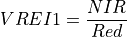
11.1.7.18. Vogelmann Red Edge Index 1
Description:
Narrowband vegetation index sensitive to chlorophyll concentration, leaf area, and water content.
The wavelengths of the NIR and Red are 740 and 720 nm respectively. Vegetation has values typically between 4 and 8.
Outputs:
A floating point datacube of VREI1 data.
References:
11.1.7.19. Vogelmann Red Edge Index 2
Description:
Narrowband vegetation index sensitive to chlorophyll concentration, leaf area, and water content.
The wavelengths of the NIR1, NIR2, NIR3, and NIR5 are 747, 734, 726, and 715 nm respectively. Vegetation has values typically between 4 and 8.
Outputs:
A floating point datacube of VREI2 data.
References:

11.1.7.20. Vogelmann Red Edge Index 3
Description:
Narrowband vegetation index sensitive to chlorophyll concentration, leaf area, and water content.
The wavelengths of the NIR1, NIR2, NIR3, and NIR5 are 747, 734, 720, and 715 nm respectively. Vegetation has values typically between 4 and 8.
Outputs:
A floating point datacube of VREI3 data.
References:

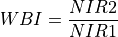
11.1.7.21. Water Band Index
Description:
Index sensitive to water concentration in vegetation canopies. Smaller numbers mean higher water content.
The wavelengths of NIR1 and NIR2 are 900 and 970 nm respectively.
Outputs:
A floating point datacube of WBI data.
References:
Penuelas, J., et al. “The Reflectance at the 950-970 Region as an Indicator of Plant Water Status.” International Journal of Remote Sensing 14 (1993): 1887-1905.
11.1.8. Clustering
11.1.8.1. HDBSCAN Clustering
Description:
HDBSCAN is a clustering tol that allows varying density clusters and does not force outliers into clusters. This is an important feature when working with noisy data. It is a multi-step algorithm summarized in 5 steps below:
Transform the space according to the density estimate.
Build the minimum spanning tree of the distance weighted graph via Prim’s algorithm.
Construct a cluster hierarchy of connected components.
Condense the cluster hierarchy based on minimum cluster size.
Extract the stable clusters from the condensed tree.
Usage:
Note: This algorithm can require long run times. Dimensionality of features should be reduced first.
Minimum Cluster Size: Sets smallest size grouping to be considered a cluster.
Minimum Samples: Sets a measure of how conservative the clustering should be. The larger the number, thr more points will be declared noise.
Outputs:
A floating point datacube containing integer cluster numbers with -1 representing noise.
References:
11.1.8.2. K-Means Clustering
Description:
Partitioning algorithm that groups each sample to the cluster with the nearest mean. Iterations then successively recompute cluster means and distances until convergence or the maximum number of iterations has been met.”
Usage:
Note: As with most clustering algorithms, dimensionality of features should be reduced first if possible.
Clusters: Number of desired clusters.
Max Iterations: Maximum iterations to be used. The higher the number the slower the run time but more accurate the results. If convergence has been met the algorithm will stop before the maximum number of iterations has occurred.
Outputs:
A floating point datacube containing integer cluster numbers.
References:
11.1.9. Mask
11.1.9.1. Apply Mask
Description:
Overlays the supplied mask on the datacube. Pixels with mask values of one get passed through where mask pixels with zeros are set to a user supplied number or cropped. If cropped, spatial relationships of the datacube will likely be lost. This is useful for creating training datacubes for other classification tools.
Masks must be the same spatial dimensions as the datacube they operate on.
Usage:
New Name: New name for resulting datacube.
Technique: For Set Unmasked to Value, masked pixels will be set to the Mask Value. If set to Crop Masked, the pixels will be cropped from the datacube, likely losing the spatial relationship of the pixels as a result. This can be used to build training datacubes for use with classification tools.
Mask Value: Value to set unmasked pixels to.
Mask Cube: Mask datacube.
Outputs: Datacube with mask applied.
11.1.9.2. Build Mask
Description:
Builds a mask to apply with the Apply Mask tool. This tool uses a threshold to partition pixels into ones or zeros. In the Apply Mask tool, the mask is overlayed on a datacube and pixels with ones get passed through where pixels with zeros are set to a user supplied number or cropped. Typically, the Build Mask tool is applied to a previously classified datacube which can be partitioned with a threshold.
Usage:
Threshold: Threshold to partition data with.
Invert: If checked, pixels above the threshold are set to zero and pixels below the threshold are set to one. If unchecked, the opposite is true.
Outputs:
A mask datacube containing ones and zeros.
11.1.9.3. Build Mask from Saturated Spectra
Description:
Builds a mask from saturated spectra to apply with the Apply Mask tool. In the Apply Mask tool, the mask is overlayed on a datacube and pixels with ones get passed through where pixels with zeros are set to a user supplied number or cropped.
Usage:
Saturation Value: Level at which saturation occurs. Defaults to the ceiling value in the header or the bit depth value if ceiling is not available. User can overide.
Invert: If checked, saturated pixels are set to one and pixels below the threshold are set to zero. If unchecked, the opposite is true (normal usage).
Outputs:
A mask datacube containing ones and zeros.
11.2. Render Plugins
11.2.1. Band Average
Description:
Averages all of the bands and displays the greyscale result.
11.2.2. Classification to Colormap
Description:
Display a unique color for each class, where pixel membership is given by the band number in which the maximum or minimum value occurs.
Usage:
Evaluate by: Choose whether class membership is evaluated by minimum value or maximum.
Colors: Click on class color button to choose color.
11.2.3. Foreground Object Detection
Description:
This powerful tool is useful for extracting objects from their backgrounds for creating training sets, making masks, or for visualization purposes.
The tool has two distinct steps. First, input the Background cube or cubes and the known options below. It will return a preview of the results, which can be used to fine tune the output. (Use the Auto Update checkbox to streamline the fine tuning process.) Once satisfied, press the Run Now button in the Export Results box.
Usage: Number of Background Cubes: The number of different background cubes. If a spectrum in the target datacube is similar to any of the background cubes, it will be considered background.
Use per-cube thresholds: If checked, each background cube will have a unique threshold slider. If unchecked, a single threshold will be applied to all background cubes.
Threshold: Threshold to fine tune the separation of foreground from background for all cubes (only visible if Use per-cube thresholds is unchecked).
Background Cube -> Cube: Select a datacube representative of the background to remove.
Background Cube -> Threshold: Threshold to fine tune the separation of foreground from background for this cube only (only visible if Use per-cube thresholds is checked).
Minimum Object Size: Smallest size in pixels for foreground object to extract. Can be used to filter out spatial noise.
Rectangular Cube: Check to preserve the spatial representation of the image and return a square cube. The background pixels needed to make a square image will be padded with zeros, which will contaminate training cubes. If Unchecked, spatial positioning will be scrambled but padding pixels are not necessary. Use this option for creating training cubes. The outline showing the foreground datacubes will disappear if this option is unchecked.
Combine Objects: Check to combine individual objects into a single datacube or mean spectrum. Uncheck to return all individuals.
Outline color: Press to select a different color to outline the results.
Morphological Opening: Erodes then dilates an image, useful for removing small objects.
Morphological Closing: Dilates then erodes an image, useful for filling small holes.
Border Pixel Erosion: Shrinks the foreground by expanding the background, removing unwanted edge pixels.
Structuring Element Size: Size of the structuring element to user in Opening, Closing, and Erosion. The larger the element, the greater the effect.
Save To Disk: Check cube and/or spectra to save them to disk. Specify directory below. Spectra are the mean spectra of the foreground objects, or mean of the combined foreground objects if chosen.
Spectrum Save Format: Select to save spectra as .spec, .txt, or .csv.
Save Directory: Directory to save results to.
Add To Workbench: Check to add datacubes, spectra, and/or mask cubes to the Spectronon Resource Tree (Workbench).
Run Now: Press button to execute.
Outputs:
Datacubes and/or spectra saved to disk (optionally)
Datacubes, spectra, and or mask cubes added to Workbench (optionally)
11.2.4. Greyscale
Description:
View a greyscale image by wavelength, band number, or band name.
Mode: Choose to view by wavelength, band number, or band name, if available.
Wavelength/Band/Band Name selector: Choose wavelength/band to view.
11.2.5. Greyscale to Single Color
Description:
Assigns a color to a single band datacube.
Usage:
Color: Select Red, Green, or Blue.
Invert: Check to make lower pixel values the brightest.
Clip Negatives?: Check to clip negative values to zero for display purposes.
11.2.6. Last Frame
Description:
View the last raw data frame of the datacube. A frame is a 2D image with a spatial dimension on one axis and spectral on the other.
11.2.7. RGB
Description:
View three bands of a datacube with a composite Red, Green, and Blue (RGB) image.
Usage:
Mode: Specify band selection by wavelength or band number.
Adjustments (Red, Green, and Blue): Select wavelength or band number for each color.
Presets: Depending on the wavelength range of the datacube, the Preset buttons will specify the above wavelengths for Red, Green, and Blue to standard wavelengths. In the VNIR, the options are True Color (normal color image) or Color Infrared (uses Green, Red, and Infrared wavelengths).
11.2.8. Raw Camera Data
Description:
View raw data frame from a datacube. A frame is a 2D image with a spatial dimension on one axis and spectral on the other.
Usage:
Frame Number: Select the frame number (line number) to view. -1 is the last frame, 0 is the first.
11.2.9. Scalar to Colormap
Description:
Assigns a unique color to each scalar value in a chosen band.
Usage:
Colormap: Choose colormap to use.
Normalize: Normalize band before assigning color.
Mode: Choose band selection by number or name.
Band: Band to visualize.
References:
11.2.10. Stack
Description:
Stack multiple images on top of one another with transparency. This can be useful to show classification results on top of the original RGB image, or show multiple classification results simultaneously.
Usage:
Stack Height: Number of images to stack.
Image: Select image to show.
Alpha: Sets transparency of the image. 1 is no transparency.
Make zero values transparent: Useful for classified or mask datacubes.
11.2.11. Threshold To Colormap
Description: Assigns colors to pixels of a datacube that are above or below a user-specified threshold. Useful for datacubes containing a continuous range of values (such as spectral angles or probability results) that must be thresholded for final classification. One user-specified threshold is available for each band of the datacube.
If multiple bands of a pixel meet the threshold requirement, the color corresponding to the largest band values that meet the threshold (in probability or above threshold mode) or smallest band values (in distance or below threshold mode).
Pixels that do not meet the requirements of any threshold are colored black.
Usage:
Classification type: Determines whether colors are assigned corresponding to pixel values above the threshold or below the threshold. In probability or above threshold mode, colors are assigned corresponding to pixel values that are greater than the threshold. In distance or below threshold mode, colors are assigned to pixel values that are less than the threshold. Probability mode sets the range of possible thresholds between 0 and 1. Distance and below threshold modes are equivalent.
Value: Threshold value.
Color: Color to assign.
11.3. Filter Plugins
11.3.1. Colormap Stretch…
Description:
Assigns a color to individual scalars in a single band image. Similar to the Scalar to Colormap Image tool.
Usage:
Use Contrast Enhancement: Check to stretch image by below method (Linear Percentage, Linear Absolute, or Histogram).
Colormap: Choose colormap to use.
Method: Choose how to stretch the data before applying colormap.
Parameters: Depending on Stretch method chosen, different parameters are available:
Low/High Cut: Choose high and low cut values to stretch the remainder through. Use Preset buttons go to default presets.
Stretch Bands Individually: Not used in this tool.
Inverse: Invert the high/low colormap scheme.
Bins: NUmber of histogram bins to use.
References:
11.3.2. Contrast
Description:
Apply a linear percentile, linear absolute, or histogram stretch to the image.
Usage:
Use Contrast Enhancement:
Check to stretch image by below method (Linear Percentage, Linear Absolute, or Histogram).
Colormap: Choose colormap to use.
Method: Choose how to stretch the data before applying colormap.
Parameters: Depending on Stretch method chosen, different parameters are available:
Low/High Cut: Choose high and low cut values to stretch the remainder through. Use Preset buttons go to default presets.
Stretch Bands Individually: Check to stretch each band by statistics of each band, uncheck to stretch all bands by statistics of all.
Inverse: Invert the high/low colormap scheme.
Bins: NUmber of histogram bins to use with the histogram stretch.
11.3.3. Gaussian Blur
Description:
Apply a Gaussian blur transformation to each pixel in the image using a kernel which can be given an independent height and width
Usage:
Use Gaussian Blur: Turns the filter on or off.
Kernal height: Height of the Gaussian blur (range 1-15, default 3), in pixels
Kernal width: Width of the Gaussian blur (range 1-15, default 3), in pixels
Border type: One of the OpenCV border types, defaults to ‘BORDER_DEFAULT’
11.3.4. Local Modal Filter
Description:
Assign each pixel to the value most frequently occurring in a local spatial window around the pixel.
Usage:
Use Modal Filter: Turns the filter on or off.
Window Size: Size of the window to evaluate most frequent value around given pixel, in pixels.
Window Shape: Shape of the window.
11.3.5. No Filter
Description:
No filter is used. Depending on the datacube values, the resulting image might appear completely dark, white, or have very little contrast on the screen.
11.3.6. Threshold
Description:
Apply a threshold to the image. Options include a simple binary threshold based on a single number, thresholding below minimum and above maximum values, and thresholding values between the minimum and maximum. Inversion of the results is also an option.
Usage:
Min Threshold:
Values below or equal to this threshold are set to white, unless thresholds are locked. If True Between is checked, values below this threshold are set to black.
Max Threshold:
Values above or equal to this threshold are set to white. If True Between is checked, values above this are set to black.
Lock Min-Max:
Locks Min and Max together. Values above or equal to this value are set to white, values below are set to black.
Inverse:
Inverts black and white.
True Between:
Sets values below Min Threshold to black, values above Max Threshold to black, and values between (including equal to) to white.
11.4. Select Plugins
11.4.1. Create Cube From Selection
Description:
Create a new cube from selection. If the selected area is rectangular, the dimensions of the selected area will be preserved. If the selection is not rectangular, the spatial relationship will be scrambled in order to make a rectangular datacube.
11.4.2. Create Mask Cube From Selection
Description:
Create a single band cube from the selection where selected areas are 1 and unselected areas are 0.
11.4.3. Mean Spectrum
Description:
Create and plot a spectrum from the mean of the selected region. Wavelength metadata must be present for this tool to be available.
The standard deviation will also be plotted, which can be turned on or off by right clicking on the Spectrum object in the Resource Tree and selecting Show/Hide Standard Deviation.
11.4.4. Show Mean of Selection
Description:
Show a dialog box with the mean of each band in the selected region. Useful for datacubes with few bands, bands that don’t contain spectral data, and/or datacubes containing disparate data.
11.4.5. Mean Z profile
Description:
Create and plot the mean profile of the selected region in the Z (band) dimension. If wavelength metadata is present this is equivalent to the Mean Spectrum tool.
The standard deviation will also be plotted, which can be turned on or off by right clicking on the Spectrum object in the Resource Tree and selecting Show/Hide Standard Deviation.
11.4.6. Mean First Derivative
Description:
Plot the mean first derivative (discrete difference) of the selected area.
11.4.7. Spectral Correlation Matrix
Description:
Creates a heatmap showing band-to-band correlations using the Pearson coefficient. The diagonal is always 1 (perfect correlation as bands are identical), while uncorrelated bands have values of zero. This heatmap may useful for exploring data qualitatively.
Usage:
Save Correlation to Disk:
Check to save.
Colormap:
Colormap to use.
References:
11.4.8. Create Correlation Coefficients
Description:
A correlation coefficient aligns reflectance data created with downwelling irradiance data to a ground truth target such as a tarp or reflectance standard. Once created, these coefficients are used in the Reflectance Conversion with Downwelling Irradiance plugins to improve the accuracy of the result.
Usage:
Start by creating a region of interest of the ground truth target.
Use Measured Reflectance:
Check to use a previously measured reflectance spectra for the reference object the region of interest contains. Uncheck to assume a flat reflectivity.
Measured Reflectance File:
Select the previously measured reflectance spectrum. The first column should be wavelength in nanometers, the second column is reflectance from 0-1 or 0-100%. File should be tab, comma, or space delimited.
Flat Reflectivity:
Select flat reflectivity of ground truth target if measured spectrum is not available or desired.
Measured Reflectivity in Percentage:
Check if measured reflectance spectrum is on the scale 0-100. Uncheck if 0-1.
Outputs:
Spectrum of correlation coefficients.
11.4.9. Find Closest RAL Classic Color
Description:
Uses spectral information to determine the closest RAL Classic color to selected region. Wavelength and reflectance scale factor metadata must be present. Useful for color matching.
References:
11.4.10. Median Spectrum
Description:
Plot the median spectrum within selected area.
11.4.11. Mean Nth Derivative
Description:
Compute and plot the mean Nth derivative (discrete difference) of the selected region.
11.4.12. Save random spectra to text file
Description:
Randomly selects pixels within the region of interest and exports their spectra (or bands) to a text file.
Usage:
Number of spectra to export:
Number of randomly selected spectra to export.
Add Wavelengths Col:
Option to add the wavelength metadata as the first column of exported data.
11.4.13. Send To Clipboard
11.4.13.1. Copy Mean as Text
Description:
Copies mean spectrum as text to clipboard for pasting into other applications.
11.4.13.2. Copy All as Transposed Text
Description:
Copies mean spectrum as transposed text to clipboard for pasting into other applications.
11.4.13.3. All Spectra as Text
Description:
Copies all spectra in region as text to clipboard for pasting into other applications.
11.4.13.4. Copy as Image
Description:
Copies image of region to clipboard for pasting into other applications.