7. Advanced Data Analysis 2: Hyperspectral Classification
7.1. General Approach
The detailed spectral information in hyperspectral data enables one to distinguish between very similar objects. Additionally, machine vision algorithms enable rapid, accurate, and repeatable classification of objects. With these capabilities, hyperspectral imaging has a broad range of current and potential applications, including sorting (food, raw materials, recycled materials), quality control (pharmaceuticals, food, printed goods), remote sensing (defense, search & rescue, mineral exploration, agriculture), to name just a few.
Critical to all of these applications is implementation of algorithms that classify the pixels within an image based on their spectral profiles. This section provides an introduction to hyperspectral data classification. There are many approaches to classifying objects. However, the general approach to most of these algorithms can be understood by considering the following simplified hypothetical examples.
In general, the algorithms used to classify objects scale with the number of spectral channels. Understanding how the general approaches work with a simple 2-color system makes it relatively easy to understand hyperspectral classification with tens or hundreds of channels. Therefore, consider a 2-color camera that provides digital numbers for how much red and how much blue is in each pixel. (Thus, this example is even easier than a conventional digital color camera that provides digital values for the three colors: red, green, and blue.)
Much like humans need to learn to distinguish between objects, classification algorithms generally also must be trained. Typically this is done by imaging samples of interest, and then using results from this “training set” to learn how to distinguish between objects in general.
As an example, assume we wish to distinguish between the three objects shown below, a red ellipse, a blue triangle, and a purple (mixture of red and blue) parallelogram. (Ignore the grey rectangles for now.) An x and y axis is drawn to provide location coordinates for each pixel.
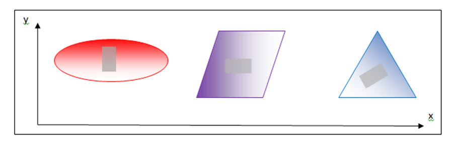
Note that each object has a distribution of light and dark pixels, although each object is approximately the same “color”. If we image these objects with our hypothetical 2-color imager that senses only “red” and “blue” channels, there will be two spectral channels per pixel. To train our imaging system, we first select a representative set of training pixels from the image of each of the objects of interest. This might be done, for example, by selecting the pixels within each grey rectangle indicated in the image above.
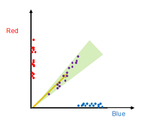
A useful way to visualize the color information in these training pixels is to plot the red and blue brightness values for each selected pixel in “color space” along blue and red axes, as shown below. (Note: This color plot uses only the training pixels selected within the three grey rectangles shown in the image above.)
We can immediately recognize the training pixels that align along the vertical (red) axis are associated with the red ellipse, as those pixels clearly have large red brightness values, but small blue brightness. Similarly, the blue triangle pixels lie primarily along the horizontal (blue) axis. The purple pixels, however, lie in between the two axes because the color purple has significant red and blue brightness (i.e., it is a mixture or red and blue). Because some of the pixels are dark and others are light, the distribution of training pixels from each object is spread out from small values to large values in a near-linear manner.
One can see that the pixels from the spectrally distinct objects are separated in this “color space”. Although this example has a 2-dimensional color space, one could create a 3-dimensional color space for RGB cameras, or 100 dimensions for 100-band hyperspectral imagers. In general, additional dimensions provide additional “opportunities” for points from different objects to be distinct in the color space, and thus they are easier to classify in practice, but otherwise the number of dimensions need not concern us now. Admittedly it is difficult to visualize a 100-dimension space, but the mathematical transition is often straight-forward. Consequently, one can invent techniques that work in two dimensions, and they can generally be applied to 100 dimensions.
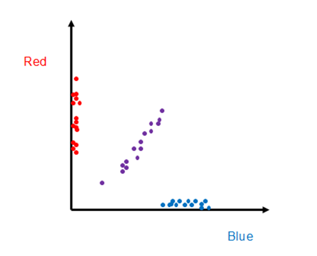
Consider the following example of the well-known hyperspectral classification algorithm known as Spectral Angle Mapper (SAM). Note that the groups of training pixels from the three different objects in our 2-dimensional color plot are located at different angles relative to the horizontal axis. The SAM technique utilizes this property to classify ALL pixels.
Consider a reference vector at the center of the group of purple training pixels. This vector is shown as a large orange vector below. Similarly, we can envision vectors from the origin to each pixel in the plot (only three are shown to reduce clutter).
One can see that the angle between the reference orange vector is small for the purple pixels, and relatively large for the red and blue pixels. Thus, if we calculate the angle between the reference orange vector and all pixels in the image, we recognize that those pixels with a small angle are from the purple parallelogram, and those pixels with a large angle from the orange reference vector are not purple pixels.
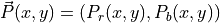
Fortunately there is an easy way to calculate the angle between two vectors by utilizing the vector dot product. To do this, write the orange reference vector in component form as

where the subscript  indicates the red brightness value component and
 indicates the blue brightness value component. Similarly, for all
pixels in the image, write
indicates the blue brightness value component. Similarly, for all
pixels in the image, write
where  and
and  indicate the location of the pixel in the original
image with an ellipse, triangle, and parallelogram. The vector dot product of
indicate the location of the pixel in the original
image with an ellipse, triangle, and parallelogram. The vector dot product of
 and any pixel
  is
is

where  and
and  are
the magnitudes of and
are
the magnitudes of and  . E.g.,
![\lvert \vec{R} \rvert = [R_r R_r + R_b R_b ]^{1/2}](_images/math/e3724d3e2833810249b82ef0e4c7cda1ee7eb93f.png) and
and
 is the angle between the reference vector
and the pixel vector .
is the angle between the reference vector
and the pixel vector .
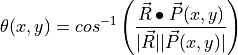
Solving for  yields
By choosing only those pixels that have an angle  (x,y) less than
some small threshold value, one can effectively identify all the purple pixels.
Graphically, this is equivalent to choosing only those pixels within a narrow
green cone, as shown below.
(x,y) less than
some small threshold value, one can effectively identify all the purple pixels.
Graphically, this is equivalent to choosing only those pixels within a narrow
green cone, as shown below.
By finding the orange reference vector and establishing the threshold of acceptable angles from this vector, we have “trained” our imaging system. To identify objects with the same color as the purple parallelogram, one images the objects and then calculates the angle as described above for each pixel. Pixels with an angle smaller than the threshold are identified to be the same material (color) as the purple parallelogram.
One could also train the system to find pixels the same color as the red ellipse or blue triangle by finding the appropriate reference vector for these objects, thereby enabling one to identify multiple objects within one image by calculating the angle between multiple object reference vectors.
To extend this approach to hyperspectral data with multiple spectral channels, one utilizes the more general definition of a vector dot product

where the sum is over all spectral bands (dimensions) indexed by  . The
angle is still the angle between the two vectors,
and , although now in a complex
multi-dimensional color space that is more difficult to visualize – the
mathematics and approach are identical.
. The
angle is still the angle between the two vectors,
and , although now in a complex
multi-dimensional color space that is more difficult to visualize – the
mathematics and approach are identical.
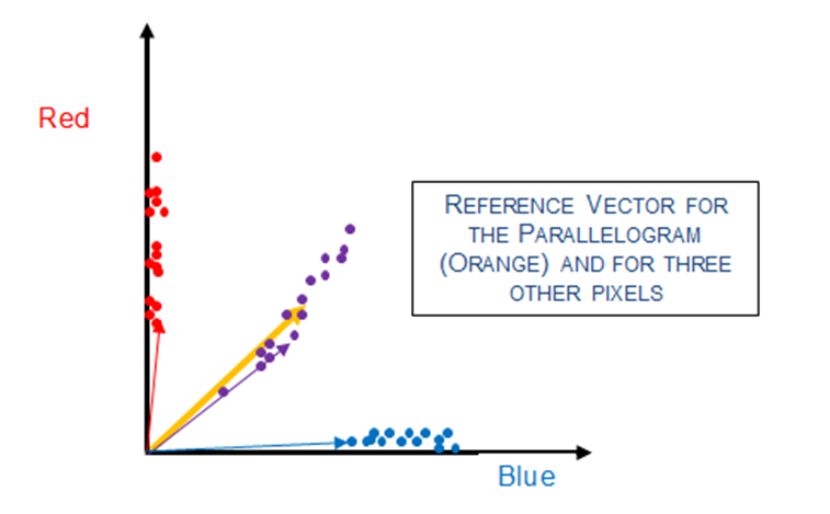
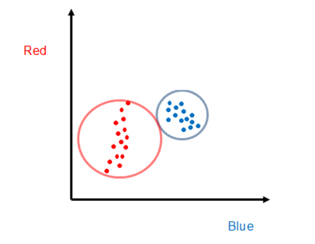
Of course SAM is not always the best algorithm to use, as one can see with the example below, where pixels from two hypothetical objects we wish to distinguish between are shown as red and blue points. In this case, if one choose representative vectors in the middle of each cluster to perform SAM classification, it is easy to see there would be substantial misclassification. (E.g., two red points lie nearly along the blue representative vector.)
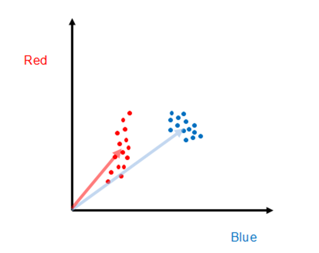
For the case shown above, a different algorithm is needed. One approach that would clearly be superior to SAM, at least for these data, is to find the center points of each set of training points, and then all points within a certain radius would be classified as that object. This is also a well-known hyperspectral classification algorithm known as Euclidean distance. Again, this approach is readily extended to hyperspectral data because the concept of distance between points is well established for multi-dimensional space.
The Euclidean distance approach can readily be improved upon by recognizing that a circle is not the best “enclosure”, and an ellipse whose axes were scaled to the point distribution width would be far better. The hyperspectral classification algorithm that utilizes this information on the distribution of training points is called the Mahalanobis distance approach. As one would expect, the cost of additional algorithm sophistication is often the need for additional processing.
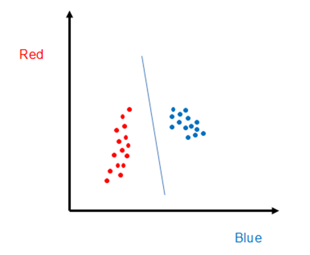
There are, of course, many other approaches to classifying objects using hyperspectral data, such as the one indicated below where one draws a line between the two sets of training points. The system is trained by noting that all pixels that map to the left of the line are associated with one object, whereas the pixels that map to the right of the line are associated with the other. Extrapolating this approach to higher dimensions is more difficult, as the line becomes a plane in three dimensions, and a hyper-plane in color spaces with dimensions larger than three.
7.2. Spectral Angle Mapper (SAM) Classification
In this example, different kinds of M&M® and Reese’s® Pieces candies are classified using the same hyperspectral datacube shown in Section 5. (This datacube can be downloaded from Resonon’s website.) To perform SAM, reference spectra must be collected for the objects of interest. In this case, based on prior knowledge, we know that the four candies indicated below (see arrows in image) are all different. Using the marquee tool or lasso, select small ROIs on each of the four candies (avoid the glare spots) indicated in the figure below. After selecting the ROI, right-click, and then select . This will generate four spectral curves in the spectral plotter, and also list the four spectral curves in the Resource Tree, as shown below.
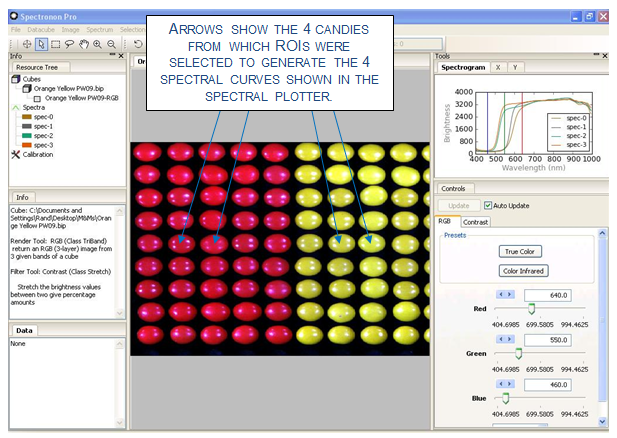
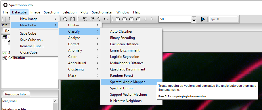
The four spectral curves shown in the spectral plotter will be used as the Reference Spectra to perform a SAM classification. To perform the classification, click on .
This will open a new window as shown. We wish to classify 4 objects, so use the slider or arrow keys to select a Spectrum for each box.
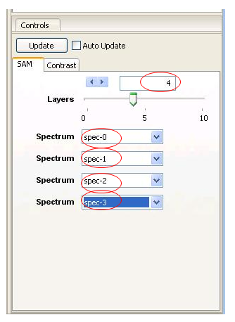
This will bring up 4 Spectrum pull-down menus. Click into each one of these and select one of the 4 spectra created with the ROI tool.
Then click OK, and Spectronon calculates the spectral angle (as described above) for each pixel for all 4 Reference spectra.
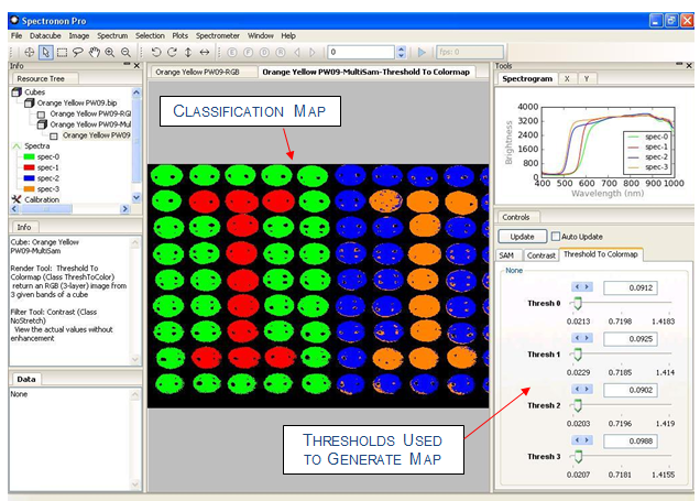
Typically, several seconds are required for the calculation, which generates a new classification map in the image panel using a default set of Threshold values.
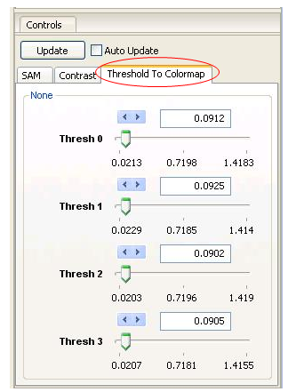
Adjust the Threshold values to obtain a more accurate classification by clicking on the Threshold to Colormap tab in the tool control panel.
To adjust the Thresholds, move the sliders, select the arrow keys, or enter values by hand. Each Reference spectrum has its own threshold. After adjusting a threshold, click Update and a new classification map will be generated in the Image panel. With a few tries, a classification rendering similar to the one shown below can be generated. Only those pixels within the threshold are colored (the classification colors match those shown in the spectral plotter and Resource Tree for the Reference spectrum). If a pixel’s Spectral Angle is within the threshold for more than one Reference spectrum, the quantity (Spectral Angle)/(Threshold Value) is calculated for each Threshold and classified for the class that minimizes this quantity. This weighting scheme allows you to emphasize or deemphasize each class to fine-tune your classification map.
SAM is only one of many, many possible classification algorithms. Other classification algorithms are accessed in a similar manner, as described in Section 11.1.2. These algorithms can be found by clicking . Additionally, user-defined scripts can be written and used with Spectronon for custom classifications algorithms.