3. Basic Data Acquisition

3.1. Data Modes and Sources

It is important to consider the data mode of the various hyperspectral imaging systems that produce hyperspectral datacubes. Hyperspectral data from Resonon imaging systems can be utilized in three forms, as summarized below. Which modes are used is application dependent, and affects subsequent datacube analyses.

3.1.1. Raw Data

These data are spectrally calibrated but are not corrected for the instrument-sensor-response or illumination functions, so the result cannot be directly interpreted as, for example, reflectivity. The units are digital number (DN) from the imager camera’s sensor array. If a dark frame has been recorded, these data may have the camera’s average dark current subtracted, but no other correction are applied. This is the least useful data form, as the spectral curves do not have physical units. Spectronon can collect datacubes in this mode with either a Benchtop System or Outdoor Field System.

3.1.2. Radiance

Raw data can be post-processed to give radiance data, where the DN unit is converted to physical units of microflicks (1 microflick = 1 microwatt per steradian per square centimeter of surface per micrometer of span in wavelength). This mode removes the imager’s instrument-sensor-response function from the data. This function is corrected for by using the Imager Calibration Pack (ICP file) with the Radiance From Raw Data plugin. The resulting data are the product of illumination and sample-reflectivity functions. In addition to the standard spectral calibration, radiance measurements require Resonon to perform a radiometric calibration (rad cal) on the imager with the desired objective-lens aperture. Radiance conversions are typically performed with Spectronon on datacubes collected under stable, uniform lighting conditions, such as with Resonon’s Outdoor Field System or Airborne Remote Sensing System.

3.1.3. Reflectivity/Reflectance

In reflectance mode, both the instrument-sensor-response and illumination functions are removed. This leaves the data in absolute reflectance. Resonon’s Benchtop System commonly performs reflectance measurements on a sample by applying a response correction that employs a separate scan of a reflectance standard that corrects for the instrument-sensor-response and illumination functions. The reflectance standard, or calibration tile (cal tile), fills the entire field of view (FOV) of the imager. Spectralon® and Fluorilon® are the highest quality reflection standards, but Teflon is acceptable for many applications. (Teflon needs to be sanded with 100 grit sandpaper on an orbital sander to eliminate any specular properties).

In other system setups, such as with Resonon’s Outdoor Field System or Airborne Remote Sensing System, data can be converted to reflectance in one of four ways described below.

1. White reference: Data can be processed to reflectance with a calibration measurement against a reflectance standard, such as used with the Benchtop System. This calibration is done with the Record Correction Cube feature, as described in Section 3.7.2: Response Correction. It is important to note that reflectance values are only accurate if the solar illumination (cloud, sun angle, etc.) does not change between the collection of the response-correction datacube and the sample datacube. Data can also be converted to reflectance using the Reflectance from Raw Data and Spectrally Flat Reference Cube plugin.

2. Known spectral reference in scene: After the data have been converted to radiance, the known spectrum of a reference object in the scene can be used to correct the rest of the cube to reflectance. The reference spectrum must be known and in a tab- or space-delimited file. Use the Reflectance from Radiance Data and Spectrally Flat Reference Spectrum plugin.

3. Downwelling irradiance sensor: An alternative method for converting data to reflectance is to use a downwelling irradiance sensor. This sensor records the solar spectrum during data acquisition. This data is used, along with the Imager Calibration Pack (ICP) file(s) supplied by Resonon for both the spectral imager and the downwelling sensor. This method uses the Reflectance from Radiance Data and Downwelling Irradiance Spectrum plugin.

4. Atmospheric Correction: Data can be converted to reflectance with the use of atmospheric correction algorithms such as FLAASH (Fast Line of Sight Atmospheric Analysis of Spectral Hypercubes). Please contact Resonon for more information.

3.2. Start The System

If you have an illumination system, turn it on and let it warm up sufficiently. Some lights may require 15 to 20 minutes to fully stabilize.

With the imager and (optional) stage connected to your computer, launch Spectronon by double-clicking on the Spectronon icon or starting Spectronon from your Start menu. The Spectronon icon and user interface are shown below with the various windows labeled.

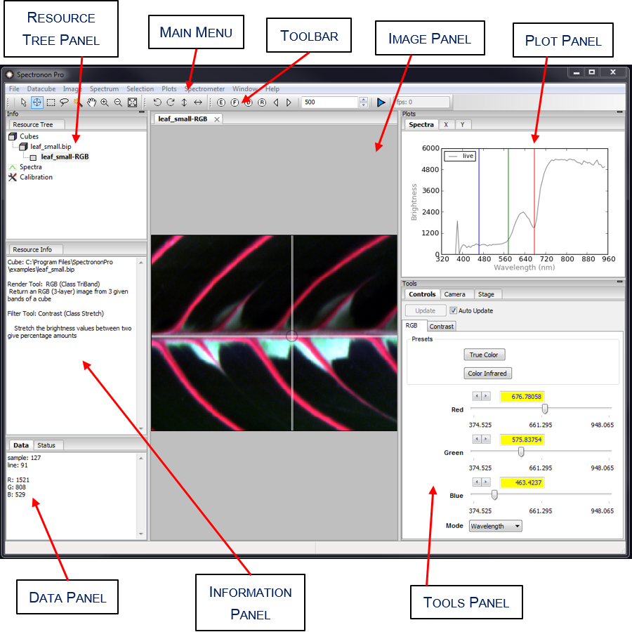
Once the software has started, make sure that the imager and stage controls (if used) are enabled, which indicates that they are properly connected. The imager and stage tools will be greyed out if not enabled, as shown below.

You can get the latest version of Spectronon by clicking on Help ‣ Check For Updates. This won’t download the latest version, but will give an alert if there is a newer version, as well as a hyperlink to it.

3.3. Verifying Imager Calibration

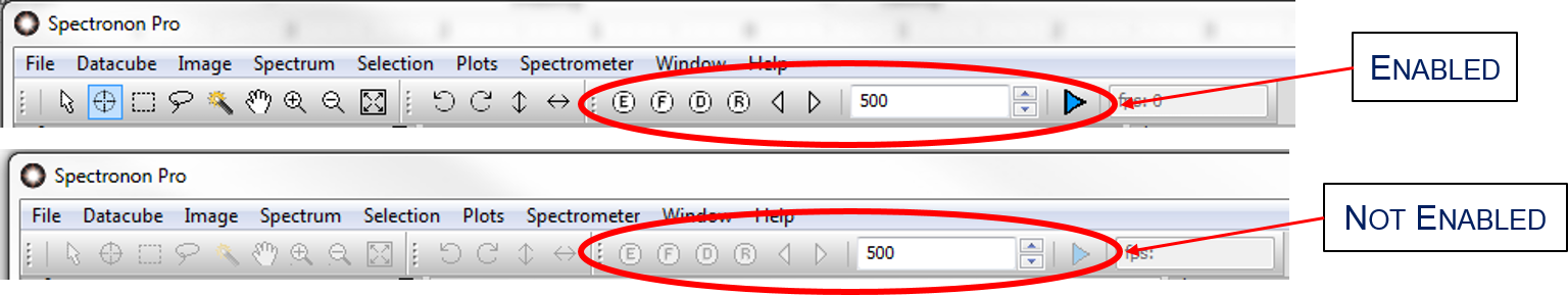
From the Main menu, select File ‣ Preferences….

This will reveal the Preferences window. This window has several tabbed panes that provide detailed information about the connected Imager and Stage, as well as settings for the Scanner, managing and analyzing datacubes on the Workbench, and visualizing data with Plotters.

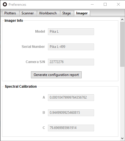
In the Preferences window, select the Imager tab to reveal detailed information about your connected hyperspectral imager. Your imager was calibrated at the factory. The spectral calibration numbers are provided on a sheet that comes with your imager and should be verified prior to use. Check the A, B, and C values from the sheet provided against the Spectral Calibration values appearing in Spectronon. If you cannot locate your calibration sheet or these numbers differ from those reported in the software, then please contact Resonon at: ProductSupport@resonon.com.

3.4. Imager Controls

Camera Settings for the imager can be controlled by clicking on the Imager tab in the Tools panel in the Main window.

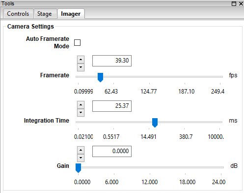
Imager Camera Settings with Auto Framerate Mode off.

Framerate is equal to the number of datacube lines acquired each second, or frames per second (fps). The Framerate limits the maximum Integration Time, where typically Integration Time 1 / Framerate.

Integration Time is the duration of data acquisition for each individual line (also known as exposure time), displayed in milliseconds (ms). Larger integration times require smaller frame rates, and smaller integration times allow faster frame rates. Integration times that are too short have poor signal-to-noise ratio. Integration times that are too long saturate pixels in the detector.

Gain is a factor that increases the signal, but at the expense of signal-to-noise ratio. Keep the gain as low as possible, preferably zero. A gain of 6 dB roughly doubles the signal. (The IR imagers do not have this setting.)

Some of Resonon’s imagers support Auto Framerate Mode. When enabled, the Framerate cannot be set directly. (However, the frame rate can still be viewed.) The user need only select an appropriate Integration Time (and Gain, possibly) based on the illumination and sample brightness, and Spectronon automatically chooses the fastest Framerate for that Integration Time. This helps produce the fastest possible scans for a given setup.

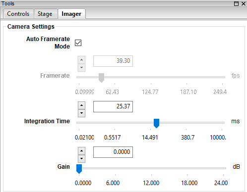
Imager Camera Settings with Auto Framerate Mode on.

Additional Imager settings are available in Preferences–>Imager, described in Section 4: Advanced Data Acquisition.

3.5. Stage Controls

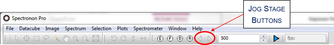
The stage is configured at the factory for either the Benchtop System (cm units) or the Outdoor Field System (deg units). You can move the stage manually by clicking on the Jog Stage buttons, located on the toolbar. The buttons move the stage incrementally in either direction. Use the buttons to center the stage underneath the Pika imaging spectrometer.

The stage can be further controlled by clicking on the Stage tab in the Tools panel. The default stage setting in Spectronon is Auto Speed Mode. This means that the Framerate of the imager’s camera is used to automatically calculate the stage’s Scanning Speed. Because the imager is a line-scan imager, the stage must traverse at a speed proportional to the camera’s framerate in order to capture the scene with a unit aspect ratio. If the stage is too slow with respect to the Framerate, then the image is elongated in the direction of stage travel. If the stage is too fast with respect to the Framerate, then the image is shortened.

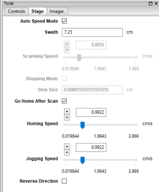
For the Benchtop System, the Swath value is key to achieving unit aspect ratio scans when using Auto Speed Mode. The swath is the width of the stage that is viewed by the imager, and is affected by the choice of objective lens and the working distance from the (in-focus) object on the stage to the imager. A procedure for determining a value for Swath is provided later in Section 3.8: Scanning and Saving Datacubes. In the Outdoor Field System, this Swath is replaced by the angular FOV (field of view), which is typically the far-field value specified for the given objective lens.

With Auto Speed Mode selected, several controls are disabled and serve only as value indicators. The Scanning Speed indicates the continuous scanning speed, and is set automatically. If the stage cannot move sufficiently slowly in a continuous manner, then Stepping Mode will be enabled. In Stepping mode the datacube is acquired line-by-line with the stage coming to a stop for each line, i.e., stepping. (Stepping occurs for a sufficiently long Integration Time corresponding to a sufficiently low Framerate.) The Step Size parameter indicates how much each line in the scan covers (continuous or stepping).

If Go Home After Scan is selected, then the stage will return to its starting position after each scan. The speed at which the stage returns to its original position is the Homing Speed. (The Homing Speed setting is also used to set the between-steps Scanning Speed when the stage is automatically put into Stepping Mode.) Jogging Speed is used for the Jog Stage buttons, described above. Reverse Direction reverses the scan direction of the stage, including the jog directions.

Additional Stage settings are available in Preferences–>Stage, described in Section 4: Advanced Data Acquisition.

3.6. Focusing Objective Lens

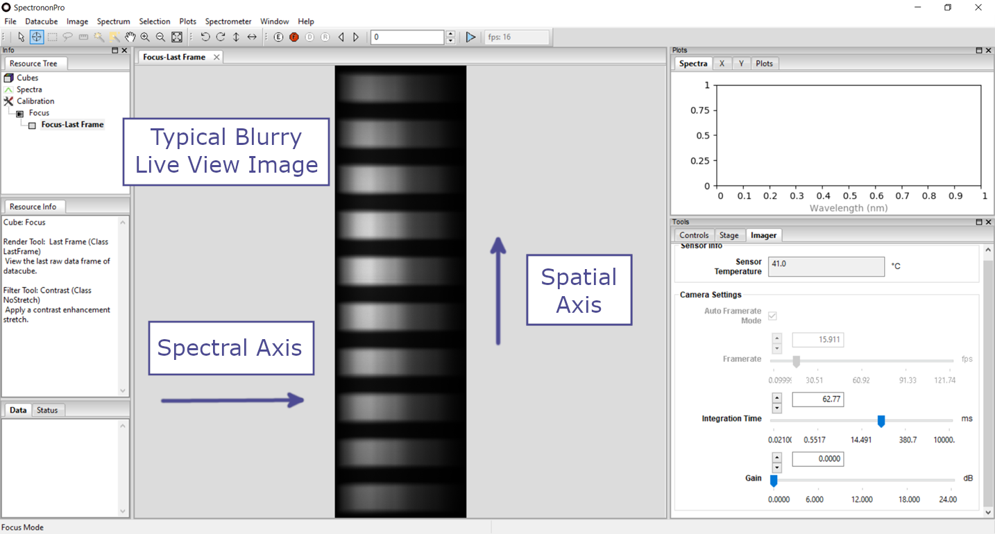
You are now ready to focus the objective lens of your Pika imaging spectrometer. At first, this process can be somewhat challenging, but with a little practice it becomes straightforward. Begin by clicking on the Focus button located on the Spectronon tool bar. This will reveal a live image of individual frames from the imager’s camera. (Wave your hand in the field of view (FOV) of the imager to confirm that the image is a live view.) One axis of this image represents the spatial (position) axis of your object, and the other is the spectral (wavelength) axis. (To understand this view better, move colored objects within the FOV of your imager after you have focused the objective lens.)

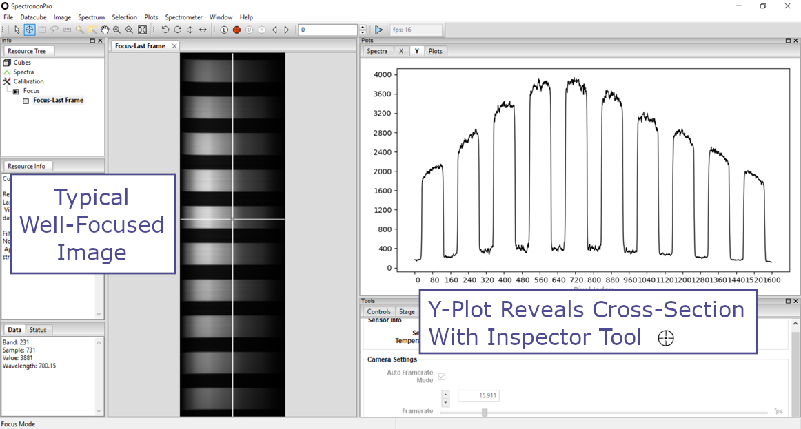
Place an object with multiple light and dark regions within your Pika imaging spectrometer’s FOV. For the Benchtop System, make sure that the illumination is adequate and sufficiently uniform, and place a sheet of paper with dark lines on the stage, as provided in Section 10: Focusing & Calibration Sheets. For the Outdoor Field System, if you are in the field and are observing objects at a distance, then direct the imager towards an object with multiple features, such as a tree with many branches. Unless your lens is already focused, you will see a series of blurry or barely discernible lines in the live-view image in the center panel of Spectronon.

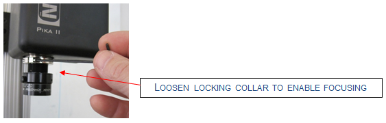
To adjust the focus, first unlock the focus adjustment. With Schneider lenses, this is done by loosening the locking metal collar on your objective lens using an Allen wrench, size 5/64 inch.

Then rotate the objective lens until you see dark lines from your object come into focus, as shown. Maximize the sharpness of the lines.

Hint

Clicking the Inspector Tool on the live view image, and then selecting X tab in the Plots window will reveal a cross-section plot of your image. Viewing this plot allows you to graphically see the sharpness of your focusing. You can zoom in on the X-axis by clicking the Zoom Tool and then clicking on the X-axis.

Note

In the Benchtop System, the working distance is often changed to fill the imager’s FOV with the sample being scanned on the stage. If you change the working distance, then you will need to refocus the imager and update the Swath value under the Stage tab in the Tools panel. A good first estimate of the value for Swath can usually be made from the ruled lines of the in-focus focusing sheet.

Focusing the Outdoor Field System can be a little more challenging than the benchtop system. If you are focusing on objects that are further than 40 feet start the process with the objective lens screwed in close to the collar. A method that has proven useful is to start the focusing process by increasing the number of lines scanned to 1000. This gives a large scan area to begin the process. You will need to be out of live focus mode when performing this focusing procedure (”F” button should not be red). When the scan begins make a quarter turn with the lens. Continue to make quarter turns until you are confident your scene is in focus. When making the quarter turn, intentionally place your hand in front of the lens. This will create a thin black line in the scan separating one focus length from its neighbor, allowing for easier comparison. This process can take some time, so be patient and remember that it gets easier with practice.

Once you have completed focusing, re-tighten the lock to the focus adjustment. Then click on the Focus tool again to toggle the camera live view off.

Note

See our YouTube video on focusing the benchtop system at https://www.youtube.com/@resonon/videos.

3.7. Reflectance Measurement Calibration

The following discussion describes how to set up your system to scan for reflectance scaled to a reference object. If you wish to collect raw data and convert it to radiance do not perform the following correction process.

Note

The Dark Current button and the Response Correction Cube button are disabled in live camera view mode. If needed, then click on the Focus tool to toggle the camera live view off.

3.7.1. Dark Correction

Spectronon can remove the imager camera’s average dark current from scans. Begin by clicking on the Dark Correction button on the Spectronon toolbar. You will be instructed to block all light entering the imager’s objective lens.

After you have the objective lens blocked, click OK as instructed. Spectronon will then collect multiple dark frames and use these measurements to subtract the average dark current from your measurements. The Dark Correction button on the toolbar will appear with a red check through it as soon as the dark frames have been collected . Once you see the red check, unblock the objective lens.

3.7.2. Response Correction

Measuring absolute reflectance of an object requires correction to account for instrument-sensor-response and spatially nonuniform illumination effects. To do this, click on the Response Correction button on the Spectronon toolbar. A message will appear telling you to place a reference material within your Pika imaging spectrometer’s FOV. The reference material should be uniform across the imager’s FOV. Examples of reference materials include Spectralon®, Fluorilon®, or sheets of white Teflon®.

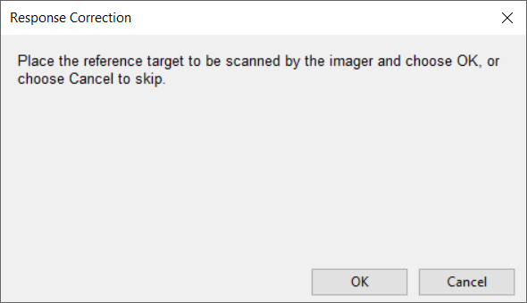
Once the reference material is in place, click on OK. This will trigger a short scan of the reference material. Once complete, the Response Correction button will appear with a red check mark , indicating that the data you collect will be scaled in reflectance with respect to the reference material, including flat-fielding to compensate for spatial variations in your lighting. Any dark correction is subtracted from the response correction.

Note

For additional help with this process see our Calibration video at https://www.youtube.com/@resonon/videos.

3.7.3. Invalidating Corrections

Once the imager is calibrated for both dark current and reflectance reference, the imager will remain calibrated until the corrections are removed by the user, or Spectronon is restarted. To manually remove the corrections, click Spectrometer ‣ Remove Dark Correction Cube and Spectrometer‣ Remove Response Correction Cube.

Dark current typically changes with the imager camera’s integration time and gain settings, the degree of which depends on the imager camera’s particular sensor. Furthermore, the response correction is likewise invalidated by changes in the imager camera’s integration time. By default, Spectronon will warn you before taking a scan if such changes have likely invalidated one/both of the corrections. Spectronon does not detect changes such as illumination and working-distance adjustments, which also invalidate the response correction.

Hint

Before collecting the dark and response correction cubes, you may first want to set the imager camera’s Framerate and Integration Time while in live view and viewing the reflectance reference. Increase the Integration Time until the signal is near, but sufficiently below, saturation over the entire frame (spatially and spectrally). Next, maximize the scan speed by choosing the fastest Framerate for that Integration Time. (If available, then Auto Framerate Mode can be turned on to have Spectronon automatically set the fastest frame rate.) Also consider the auto expose feature accessible as the Auto Expose button in the toolbar in the Scan toolbar and described further in Section 4.1: Imager Controls.

3.8. Scanning and Saving Datacubes

3.8.1. Scanning with Unity Aspect Ratio

A distortion-free hyperspectral datacube with a unit-aspect-ratio image is achieved when the stage/object advances the distance of the projected image of one spatial pixel per each line acquired at the imager’s given frame rate. Thus, changing the Framerate setting requires updating the stage’s Scanning Speed to maintain unity aspect ratio, while changing only the Integration Time does not. Similarly, changing the working distance of the imager to the stage changes the object magnification (and FOV or swath width), and thus changes the aspect ratio for any particular Framerate and Scanning Speed combination.

Hint

Typically, you want the fastest frame rate possible that supports the integration time required for the illumination and sample brightness. This is because faster frame rates produce faster scans.

By default, Spectronon has Auto Speed Mode enabled, which automates required Scanning Speed adjustments each time the Framerate changes. This depends on a single calibration parameter, the Swath setting (in cm) for the Benchtop System, or the FOV setting (in deg) for the Outdoor Field System. Once this parameter is properly “tuned” for a given system setup, you can freely adjust the Framerate without having to manually update the Scanning Speed, which is updated automatically. For very low frame rates (long integration times), Spectronon automatically compensates by turning on Stepping Mode and setting the proper Step Size.

3.8.1.1. Benchtop System

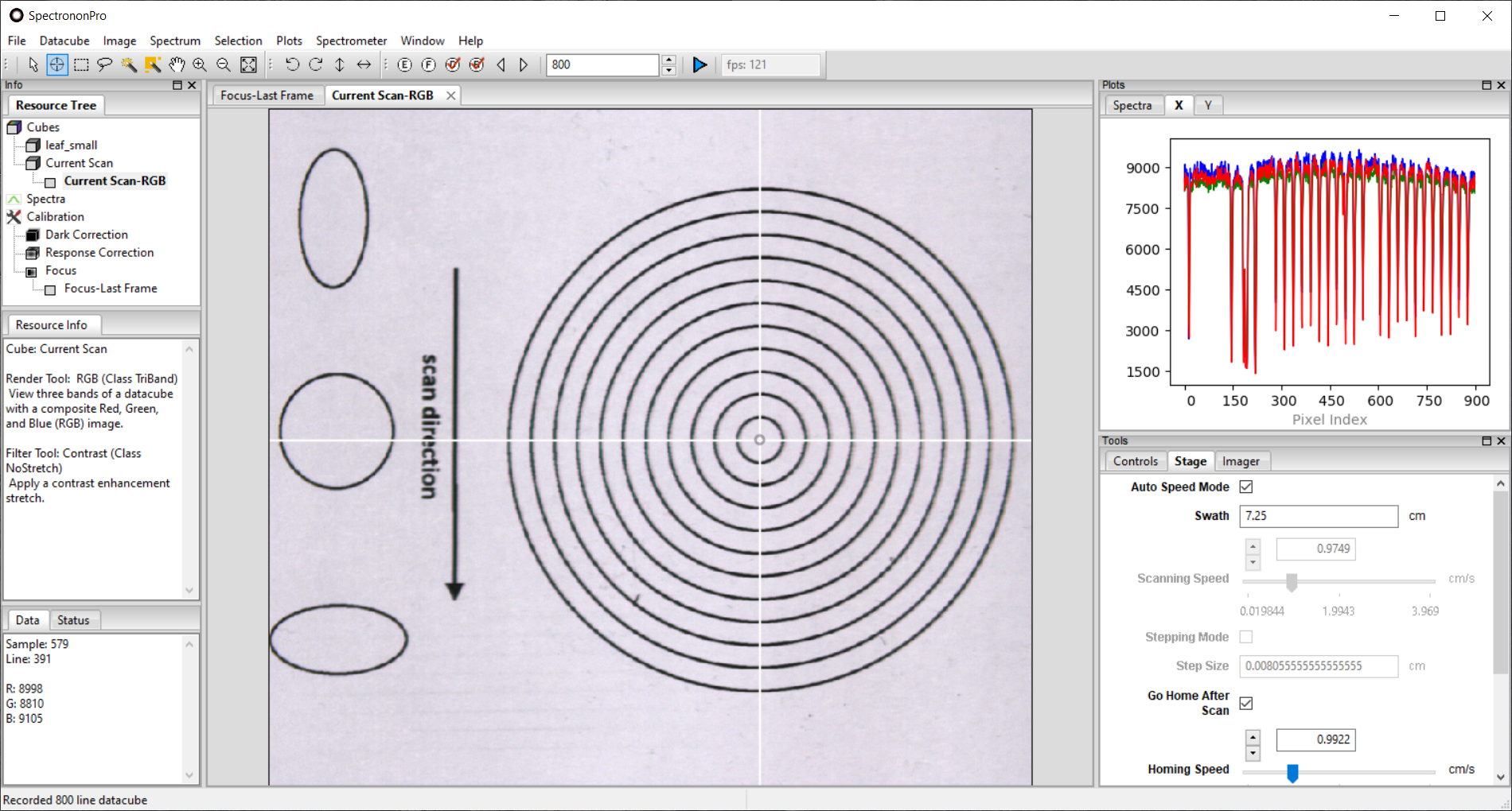
To determine the Swath setting for the Benchtop System, it is useful to first scan an object whose distortion is easy to observe, such as a circle. Print out the Pixel Aspect Ratio Calibration Sheet provided in Section 10: Focusing & Calibration Sheets for this purpose. After placing an object with circles within the FOV of your imager, record a scan with enough lines that you can see the complete circle. (500-800 lines are usually sufficient.) Record the scan by clicking on the Scan Button , and a waterfall RGB image should appear in the Image Panel of Spectronon. You may need to record several trial images to determine how many lines to scan and where to best position the object.

Hint

Stop a scan by re-clicking on the Scan Button , which changes to the Stop Button during the scan.

If the aspect ratio of the image is distorted, then you will need to change the Swath setting on the Stage tab on the Tools panel. If your image is elongated along the scan direction, then the stage was moving too slowly in relation to the frame rate (over-sampling), and you should increase the Swath setting, which automatically increases the Scanning Speed. Conversely, if your image is compacted along the scan direction, then the stage was moving too quickly in relation to the frame rate (under-sampling), and you should decrease the Swath setting, which automatically decreases the Scanning Speed. Repeat the above process until your image is no longer distorted, as pictured below.

It is also possible to measure the swath directly by imaging the vertical lines of the provided Section 10: Focusing & Calibration Sheets. Count the number of lines, and use the width between each line to estimate the total width, which is the swath width. This can even be done at the end of the imager focusing described in Section 3.6: Focusing Objective Lens.

3.8.1.2. Outdoor Field System

To determine the FOV setting for the Outdoor Field System, simply use the (far-field) FOV value specified for the imager’s objective lens, which assumes the objective lens is focused at infinity.

Note

For help setting the aspect ratio without using Auto Speed Mode see our Setting Aspect Ratio video at https://www.youtube.com/@resonon/videos.

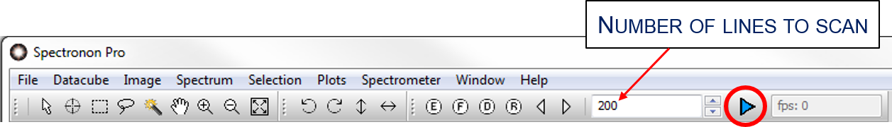
3.8.2. Scanning Objects

To scan an image of an object after calibrating the system, place the object on the stage within the imager’s FOV and type in the number of lines you would like to scan in the window just to the left of the Scan Button . Record a hyperspectral datacube (the image) by pressing the Scan Button . (Click to terminate the scan early, if needed.) Adjust the stage position and increase/decrease the number of lines as needed to cover the object’s feature(s) of interest.

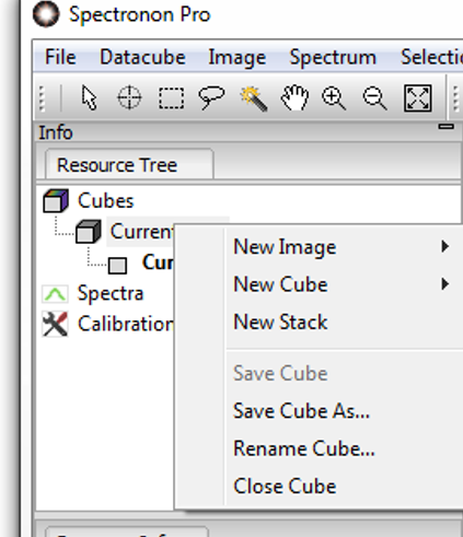
A waterfall image of your datacube will appear in the Image Panel of Spectronon, and a new entry labeled Current Scan will appear in the Resource Tree. To save the scanned datacube, use your mouse to select Current Scan and then either right-click or select Datacube ‣ Save Cube. This will open a dialog window that allows you to name the datacube and save it in a folder of your choosing. If you do not save your datacube, the current scan will be overwritten when you record another datacube, and a warning should appear.

Hint

For additional help scanning and saving datacubes see our Scanning and Saving video at https://www.youtube.com/@resonon/videos.

Once a datacube is scanned, you can use all the visualization and analysis tools of Spectronon[Pro] on your datacube image, as introduced in Section 5: Basic Data Analysis.