
7. Advanced Data Analysis 1: General
A complete listing and explanation of Spectronon’s data visualization tools is presented in this chapter. The organization of this chapter follows the main menu buttons.
7.1. File Menu
7.1.1. Open Datacube:
Clicking this option will open a window that allows you to browse and select the datacube you wish to work with. Only ENVI® compatible files will appear. Once selected, click Open, and the datacube will be loaded and an image will be generated in the image panel.
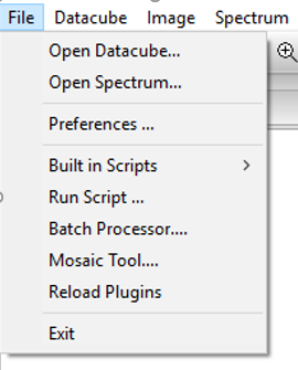
7.1.2. Open Spectrum
Clicking this option will open a window that allows you to browse and select a saved spectrum. To see how to save a spectrum, see Save Spectrum.
7.1.3. Preferences
Clicking this option opens a window that allows you to set a variety of preference options. Options associated with data visualization can be found under the Plotters and workbench tabs at the top of the window.
The Plotters tab opens a window that allows you to control the presentation of the plots presented in the spectral plotter. Additionally, this window also allows you to set the parameters for exporting plot data so it can be manipulated or plotted using other software tools.
The workbench tab opens a window that allows you to set the Default Image preference. One of the most useful settings is RGB, which generates a Red-Green-Blue image based on the values of three chosen hyperspectral bands, which you can choose in the tool control panel. Selecting the True Color button in the tool control panel produces an image that approximates the colors you would see looking at the object. Adjusting the sliders allows you to generate false-color images. Be sure to click Update after adjusting the sliders. Grayscale is another useful option, which presents a grayscale (black and white) image based on a single hyperspectral band. Again, you can adjust this band using sliders in the tool control panel. Be sure to click Update after moving a slider.
Hint
Check the Auto Update box in the tool control panel so you do not have to continually click Update.
You may find this option is too slow for large datacubes. You can also choose to open your datacubes in computer memory or your disk drive under the workbench. Generally, opening a datacube in memory is faster, but for large datacubes, or for computers with limited RAM, you may find that you need to choose the disk option.
7.1.4. Built in Scripts
Spectronon enables you to run scripts to best suit your application. A variety
of scripts are built in to Spectronon, and can be found
in File  Built-in Scripts.
7.1.5. Run Script
You may also run Python scripts you write. The Run Script opens a window that allows you to browse to your script. Additional information on how to write Python scripts for your particular need is provided in Chapter 10.
7.1.6. Batch Processor
For information on Batch Processing your data go to Chapter 11: Batch Processing of this manual.
7.1.7. Mosaic Tool
The mosaic tool is designed for an airborne application and requires georegistered data to operate. This allows the user to create one image by merging several individual images from a raster dataset.
7.1.8. Reload Plugins
When writing or changing existing plugins, clicking this will make Spectronon aware of the changes.
7.1.9. Exit
Clicking on the Exit option closes Spectronon.
7.2. Datacube Menu
7.2.1. New Image
This option allows you to create a new image in the Image panel. When you click on New Image, a menu opens three options, RGB, Grayscale, and Raw Camera Data.
Datacube New Image RGB
Generates a color image based on three bands of your hyperspectral data. These bands can be chosen and adjusted using sliders in the tool control panel.
Datacube New Image Grayscale
This produces a single-band image from a single hyperspectral band that can be chosen using a slider in the tool control panel.
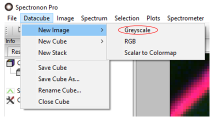
Datacube New Image Scalar to Colormap
Generates a false color image from a single band that can be chosen using a slider in the tool control panel. The colormap dropdown menu allows you to choose from a variety of color themes.
7.3. New Cube
7.3.1. Utilities
The Utilities option allows you to generate a new, modified datacube from the currently open datacube. A few of the more commonly used utilities are explained below.
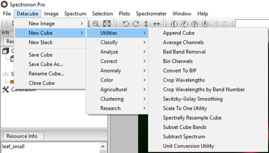
Datacube New Cube Utilities Bin Channels
Generates a new cube by binning spectral and/or spatial channels, which is often useful to either reduce the size of the datacube or improve the signal-to-noise ratio. This choice creates a new image in the Images Window and also generates a Bin Cube tab in the tool control panel with 3 sliders. The Sample Bin and Line Bin allow you to bin pixels along a spatial (x,y) axis. The Sample axis refers to the cross-track axis of the imaging spectrometer, and the Line axis refers to the along-track axis of the imaging spectrometer. The Spectral Bin slider allows you to bin spectral channels, and is likely the most useful of the binning options. After clicking Update, a new binned datacube is generated.
Note: The binned data are averaged and thus do not change significantly in amplitude. If you choose Float Mode the data will be rescaled with 1 set to the maximum bit level of the data. If your data have been scaled to a reflectance reference, you will find that glints can create Brightness values larger than one.
Datacube New Cube Utilities Crop Wavelengths
Generates an image in the Image panel and a new tab with sliders in the tool control panel that allow you to crop wavelength bands by choosing a new minimum and maximum wavelength within the cube. Once chosen, click the Update button.
Hint
You may want to click on the RGB tab in the tool control panel to reset the bands used to create the image after cropping wavelengths.
Datacube New Cube Utilities Subtract Spectrum
Generates a new cube by subtracting a background spectrum from all pixels in the datacube. This option is useful, for example, if you are monitoring fluorescent dyes and wish to subtract the background fluorescence of the substrate.
7.3.2. Classify
The Classify option allows you to generate classification maps of different objects within your hyperspectral data. More information on hyperspectral classification can be found in Chapter 8.
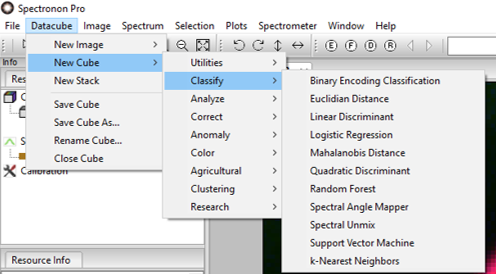
Some of the classification algorithms (SAM, Euclidean Distance, Spectral Unmix) use Spectrum objects as inputs, while the statistics-based classifiers (Logistical Regression, Quadratic Discrimient, Support Vector) require datacubes of the classification target. These are made by selecting the ROI with the lasso or marquee tool, then selecting Create Cube from Selection.
When you select one of the classification options, (e.g. SAM), a new cube will
be generated in the datatree panel. In many plugins, you will need to specify how many Layers you wish to classify (i.e., how
many materials you wish to classify) – you will then need to select a Spectrum or Cube
for each of these Layers in a pull-down menu. The Spectra and Cubes available in the
pull-down menu can be generated either by using one of the ROI tools, marquee
or lasso. ( or
or  ) or by loading a previously saved
spectrum or cube.
) or by loading a previously saved
spectrum or cube.
Note: a detailed discussion of hyperspectral data classification is beyond the scope of this document. Spectronon provides some of the more commonly used algorithms. For more advanced algorithm capability, please see other packages such as ENVI®. Additionally, custom algorithms can be utilized with Spectronon using the scripting capability described in Chapter 9. The classification options provided are:
Datacube New Cube Classify Binary Encoding Classification
The binary encoding classification technique encodes the data and endmember spectra into zeros and ones, based on whether a band falls below or above the spectrum mean, respectively.
Datacube New Cube Classify Euclidian Distance
This is a commonly used classification algorithm for hyperspectral data that is more sensitive to pixel brightness than SAM.
Datacube New Cube Classify Spectral Angle Mapper (SAM)
The SAM classification routine is described in detail in Chapter 6.
Datacube New Cube Classify Spectral Unmix
Spectral unmixing deconvolves the signal in each pixel into a linear combination of known spectra.
7.3.3. Analyze
The Analyze option allows you to perform useful operations on hyperspectral data that will generate new datacubes based on applying analytical functions to your datacube.

Datacube New Cube Analyze First Derivative
This tool generates a
new datacube with the first derivative of the spectral curve for each pixel. A
new image of the first derivative datacube is presented in the Image panel. To
see the spectral derivatives, utilize the inspector tool  , or
use one of the ROI tools marquee or lasso ( or ). The
first derivative curves appear in the spectral plotter.
, or
use one of the ROI tools marquee or lasso ( or ). The
first derivative curves appear in the spectral plotter.
Datacube New Cube Analyze Principal Component Analysis (PCA)
A detailed discussion of PCA is beyond the scope of this document (see, for example,
Wikipedia for a discussion). This tool generates a new datacube and image with
the principal component values for each pixel. Additionally, a PCA tab appears
in the tool control panel with a slider that allows you to select the number of
Bands, or PCA components. To see the PCA component magnitudes, utilize the
inspector tool , or use one of the ROI tools marquee or lasso.
( or ). The PCA magnitude curves appear in the
spectral plotter. As with standard hyperspectral data, classification
algorithms can be performed on the new PCA datacube.
7.3.4. Correct / Calibrate data
The Correct option allows you to correct / calibrate a datacube from a measured reference. This tool also allows you to convert your data to either radiance or reflectance values, as described below.
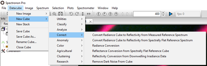
7.3.4.1. Convert Radiance Cube to Reflectivity from Measured Reference Spectrum
This plugin corrects data by using the known reflectance of an object in the scene. This requires an independent measurement of the object’s reflectance, typically obtained with a point spectrometer. This option is useful for obtaining reflectance measurements during field deployments.
This plugin applies the same calibration equally for all spatial channels in the datacube, and does not account for spatial variations in the hyperspectral camera’s response. Before using this plugin the data should be corrected for spatial variations in the camera response by converting the data to radiance using radiometric calibration. Radiance conversion is discussed below.
To use, first obtain an independent measurement of the reference object’s reflectivity, and save it as a tab delimited text file.
Next, while visualizing the data in Spectronon software, obtain a mean spectra of the reference object using the ROI tools , marquee or lasso, ( or ).
Then select Datacube
New Cube Correct
Convert… From Measured Reference Spectrum Use the Measured Reflectivity button to select the
tab delimited file of measured reflectivity. Choose the object’s mean spectrum in the “ROI Spec.” dropdown menu.
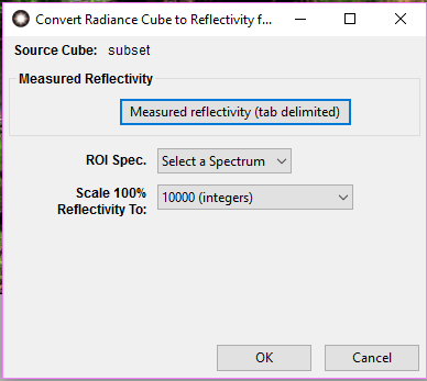
Clicking “OK” will generate a new datacube scaled to brightness values of your Correction Spectrum. If you choose 1.0 (floats) the brightness values will be scaled to “1.0” The data can also be scaled to 10,000 or the Effective Bit Depth of your camera.
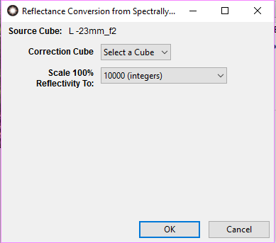
7.3.4.2. Convert Radiance Cube to Reflectivity from Spectrally Flat Reference Spectrum
This plugin also corrects data by using the known reflectance of an object in the scene, but does not require an independent measurement of the object’s reflectance by the user. The reflectivity of the object is obtained from the manufacturer, for example a tarp with a known reflectivity of 22%. This tool makes the assumption that the reference object has a flat spectral profile at a provided reflectivity. This option is useful for obtaining reflectance measurements during field deployments.
This plugin also applies the same calibration equally for all spatial channels in the data, and does not account for spatial variations in the hyperspectral camera’s response. Before using this plugin the data should be corrected for spatial variations in camera response by converting to radiance using the radiometric calibration data or ICP file (See Radiance Conversion).
To use, first obtain a mean spectra of the reference object using the ROI tools, marquee or lasso, ( or ).
Then select Datacube
New Cube Correct
Convert… From Spectrally Flat Reference Enter in the percentage reflectivity (0-1) of the reference material in the box above “Flat Reflectivity” and choose the object’s mean spectrum in the “ROI Spec.” dropdown menu.
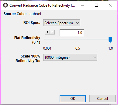
Scale the reflectivity to the selection of your choice and press “OK”.
7.3.4.3. Radiance Conversion
This plugin requires an Imager Calibration Pack (ICP File) obtained from Resonon and will return radiance in units of microflicks.
To use, select the raw datacube you wish to convert, left click, then select Datacube
New Cube Correct Radiance Conversion. The name of the raw datacube you selected will appear at the top of the pop-up window as the “Source Cube:”. Browse for the ICP file and select. It is important to note here that you should select the entire folder. All the files within this folder are necessary to perform the correction. Check the Auto Remove Dark Noise? box if you did not remove the dark noise prior to collecting the raw data and click “OK”.
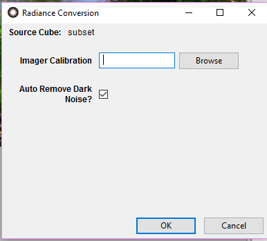
A new datacube will appear in the resource tree with your raw data converted to radiance in units of microflicks.
7.3.4.4. Reflectance Conversion from Spectrally Flat Reference Cube
This plugin allows the user to scale their raw datacube to another known reference datacube. This plugin assumes the material you used to create the datacube is 100% reflective (i.e. Teflon or Spectralon ®). It is very important that the material you are using fills the entire FOV of the camera when the cube is generated.
This plugin applies the same calibration equally for all spatial channels in the datacube, and corrects for illumination, along with spacial variations in the hyperspectral camera’s response. Making it unnecessary to convert data to radiance.
To use, the reference cube must be present in the resource tree. In the Correction Cube window, select the cube you wish to correct to. Typically this is a datacube you have recorded of a uniform reference material.
Once you click OK a new datacube will be generated that is scaled to the reference datacube and be in units of reflectance. |
7.3.4.5. Reflectivity Conversion from Downwelling Irradiance Data
This plugin is intended for data collected with the Resonon airborne hyperspectral imaging system. It requires a spectral imager radiometric calibration cube, downwelling irradiance data relevant to the datacube being collected, and downwelling irradiance sensor radiometric calibration. Optionally, dark current data for the spectral imager and downwelling irradiance sensor can be used if the dark current for these systems is significant. The returned data will be in units of reflectivity from 0-1 for float mode or 0-1000 in integer mode.
7.3.5. Anomaly
Anomaly detection tries to determine anomalous outliers in a datacube that do not conform to the expected spectra. This is usually based on a datacube of ‘clutter’, which contains the expected spectra.
7.3.6. Color
The Color option allows you to transform your hyperspectral data into CIE colorspace, providing XYZ, xyY, and LAB values for each pixel. Additionally, you can determine the ΔE values for each pixel as compared to a standard set by the user.

To transform the hyperspectral data into CIE Colorspace, choose the pathway
Datacube New Cube Color
CIE Colorspace Conversion.
This will generate a new datacube with CIE colorspace values for each pixel as
well as a new CIE Colors pace Conversion tab in the tool control panel. In this
window you are provided with standard options for the Observer and
Illumination. To see the Color space Values, position the inspector tool
on a pixel, and its values will appear in the Data panel.
Note: A warning will appear if your datacube does not have all the spectral values needed to perform a CIE color space conversion (380 nm to 720 nm). Click “ok” and Spectronon will utilize the bands available to make the appropriate conversion based on the data available.
You can determine how close the pixels are to desired Color space values by
using the ΔE option. To do this, you first have to perform the CIE Color
space conversion, as described above, then follow the path Datacube
New Cube Color
Delta E*
This will generate a new image in the Image panel and a new tab in the tool
control panel called
Delta E*. A slider appears in the tool control panel that allows you to select how many ΔE values you wish to compute. Below this, sliders appear that allow you to set your target LAB values. After setting your target LAB values, click Update. This will update your image. Use the inspector tool to see the ΔE values in the Data panel. To obtain a visual representation of the ΔE values, click on the Threshold
to Colormap tab in the parameters window and adjust the thresholds.
7.3.7. Agriculture
This option allows the user to create maps of Hyperspectral Vegetation Indices (HVI’s). HVI’s in Spectronon are discussed in greater depth in Chapter 9.
7.3.8. Clustering
Clustering tools are unsupervised classification routines that do not require any a priori information of a spectral image. They group the scene into clusters based on spectral similarity. Supervised classification routines can almost always produce better results, if scene knowledge available.
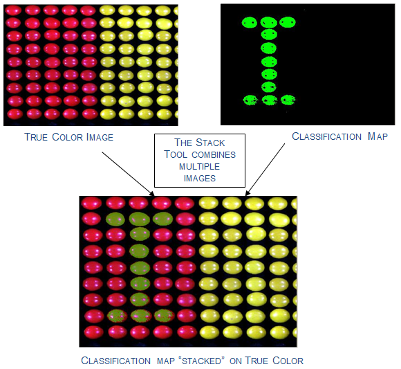
7.4. New Stack
This tool enables you to overlay multiple images. This tool is particularly useful for presenting classification results. For example, we may have a True Color RGB image of an object, such as shown below, as well as a classification map of one of the candy types. Using the Stack tool, we can combine these images to show the classification map on top of the RGB True Color image.
To use the Stack tool, follow the path Datacube
New Stack. This will open a Stack tab in the tool control panel. Use the
slider to select how many images you wish to combine (Stack height). Then click
Update. Pull-down menus appear that allow you to select the images you wish
to combine. A slider (Alpha) is available for each image that allows you to set
its transparency in the combined image. Once set, click Update and your
combined image will appear.
Tools for saving and closing datacubes are under the Datacube main menu option.
7.4.1. Save Cube
This tool will save the datacube currently open. Since many datacubes can be open at the same time, be sure to select the cube you wish to save in the Resource Tree before clicking on Save Cube. If the datacube has not been previously saved, a window will open that allows you to rename the datacube and save it in a file of your choosing.
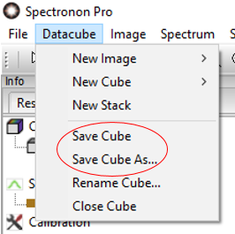
7.4.2. Save Cube As
This tool allows you to save the currently open datacube under a new name or to a new location. Clicking on this option opens a window that allows you to name the datacube and save it in a file of your choosing.
7.4.3. Rename Cube
Use this to rename datacubes.
7.4.4. Close Cube
The tool closes the datacube selected in the Resource Tree. If this datacube has not been saved, a message will appear asking to confirm whether or not you want to close it. Clicking OK will close the datacube. Clicking Cancel will cancel the command so you can continue working with the datacube or save it.
7.5. Image Menu
The Image menu provides tools for saving or closing images generated from your datacube.
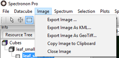
7.5.1. Export Image
Clicking on Export Image… will open a window that allows you to name and save the image file at a location of your choosing. Additionally, you can choose your preferred image format. Options include: TIFF, PNG, BMP, JPG, and GIF.
7.5.2. Export Image as KML
This allows the user to export an image in Keyhole Markup Language (KML) format.
7.5.3. Export Image as GeoTiff
This allows the user to export georegistered information within a Tiff image files.
7.5.4. Copy Image to Clipboard
This allows the user to export an image to the clipboard and paste the image into the program of their choice.
7.5.5. Close Image
This tool will close the image shown in the current Image panel.
7.6. Spectrum Menu
The Spectrum menu provides tools for manipulating individual spectrum.
7.6.1. Save Spectrum
The Save Spectrum tool will save the spectrum selected in the Resource Tree in its current configuration. If the spectrum has not been previously saved, a window will open that allows you to rename the spectrum and browse to save it in the file of your choosing. Once saved, the new name will appear in the spectral plot panel. The color selected for the spectrum will be saved.
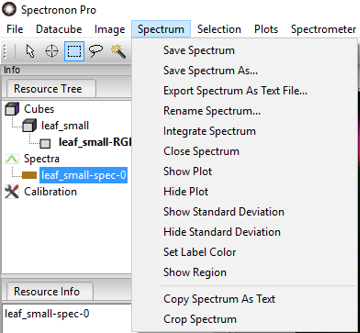
7.6.2. Save Spectrum As
This tool allows you to save a spectrum in a filename of your choice.
7.6.3. Export Spectrum as Text File
This tool allows the user to save a spectrum in a text file.
7.6.4. Rename Spectrum
This tool allows you to rename a spectrum.
7.6.5. Close Spectrum
This tool will close the spectrum selected in the Resource Tree and remove the plot from the spectral plotter.
7.6.6. Show Plot
This tool will plot the spectral curve in the spectral plotter selected in the Resource Tree. Typically this option is used after you have hidden the plot with the following Hide Plot option.
7.6.7. Hide Plot
This tool will hide the spectral plot shown in the spectral plotter. To use this tool, select the spectrum you wish to hide in the Resource Tree, and then click Hide Plot.
7.6.8. Show / Hide Standard Deviation
This tool allows you to choose whether you want to Show or Hide standard deviations when plotted.
7.6.9. Set Label Color
This tool allows you to change the color of spectral curves as well as classification maps generated with the spectral curves. To change colors of spectral curves, select the spectral curve you wish to change in the Resource Tree. Clicking on Set Label Color will reveal a pallet of colors. Choose a new color and then click “OK” and the color will be reset.
7.6.10. Show Region
Use this tool to reveal the ROI region for the plot.
7.6.11. Copy Spectrum as Text
This tool allows you to easily transfer the spectral data to another program such as Excel or Notepad. Select the spectrum you wish to copy in the Resource Tree, and then click on Copy Spectrum as Text. This copies the spectral data onto your clipboard. You can now paste the data into a program of your choosing.
Hint
Positioning your mouse on a spectrum in the Resource Tree and right-clicking will open the Spectrum menu items described above.
7.6.12. Crop Spectrum
To use this tool, first select a spectrum, then select a region in the spectra window, and then click Crop Spectrum. The result will be a graph of the spectra in the region chosen. Note this tool can be accessed by right clicking the mouse after selecting a spectra.
7.7. Selection Menu
The Selection menu items provide a number of options for use with the
selection tools (, , or  ). For all of the
following options, you must first select a Region of Interest (ROI).
). For all of the
following options, you must first select a Region of Interest (ROI).
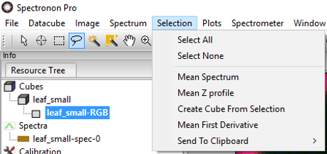
Note: The Selection menu can be accessed from the main menu or by right-clicking in the image after creating an ROI.
7.7.1. Select All
This tool selects the entire dataset.
7.7.2. Select None
This tool clears the current selection.
7.7.3. Mean Spectrum
This tool will calculate and plot the Mean Spectrum in the spectral plotter for the pixels selected in your ROI. A plot color will be automatically assigned to the plot, and the spectrum will be listed in the Resource Tree.
7.7.4. Mean Z profile
This tool will calculate and plot the mean in the spectral plotter in the Z direction if that direction is no longer wavelength and the Mean Spectrum is not available. For Example, if you performed an analysis such as CIE colorspace conversion and wanted to find the mean of a ROI from that datacube.
7.7.5. Create Cube From Selection
This tool will generate and display a new datacube from the selected ROI. An image of your new datacube will appear in the Image panel and the new datacube will be listed in the Resource Tree. This tool allows you to easily crop your datacube into smaller pieces when you wish to concentrate on small regions of your original image, or to create complete new cubes of regions of interest for quantitative analysis. If the selected ROI is not rectangular, spectronon will create a rectangular representation of the pixels within the selected ROI. The broadcast of non-rectangular ROI to a rectangular shape may result in loss of spatial information, but all spectral information will be retained.
7.7.6. Mean and Standard Deviation
This tool is much like the Mean Spectrum option, except that it will also plot curves in the spectral plotter corresponding to the mean spectrum plus and minus the standard deviation of the brightness values within the ROI. This option enables easy visualization of the variability in your spectral data as a function of wavelength.
7.7.7. Mean First Derivative
This tool plots the first derivative of the mean spectral curve within the ROI as a function of wavelength in the spectral plotter, and also lists the curve in the Resource Tree.
Hint
You may want to close all other spectra before using the Mean First Derivative tools, as the magnitude of the derivative values will typically be very different than the values of the spectra themselves.
7.7.8. Send to Clipboard
This tool allows you to transfer the data within your selected ROI. The first option is Copy Mean as Text, which allows you to paste the mean spectrum values into other applications such as Notepad or Excel. The second option, All Spectra as Text copies the spectral curves of all the pixels within your selected ROI. This tool is useful for those who want to perform specific statistical analysis on the data from small regions.
7.8. Plots Menu
The Plots menu items provide tools for the data shown in the spectral plotter.
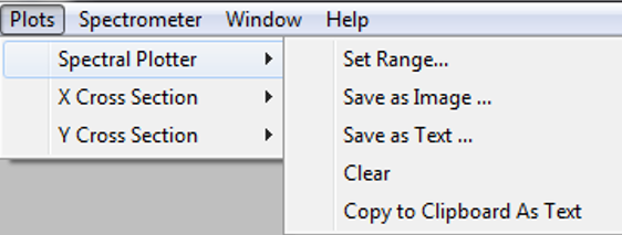
7.8.1. Set Range
This allows the user to set the range of the X-axis and the Y-axis.
7.8.2. Save as Image
This tool allows you to save the plot as an image file. Clicking on this option will open a window that allows you to name the file, select the image format, and save the plot image file in a location of your choosing. This option is available for the Spectral Plotter, X Cross Section plot, and the Y Cross Section plot.
7.8.3. Save as Text
This tool allows you to save the plot data values as a .txt file. Clinking on this option will open a window where you can name the file for the .txt file and save it in allocation of your choosing. This option is available for the Spectral Plotter, X Cross Section plot, and the Y Cross Section plot.
7.8.4. Clear
This tool allows you to remove a spectral plot. To use this tool, select the
Plot you wish to remove in the Resource Tree, then select Plots
Spectral Plotter Clear
7.9. Datacubes and Header Files
Datacubes collected with Resonon imaging spectrometers require two files, one that contains the hyperspectral data, and also a header file that contains important information about the data. Hyperspectral data can be accessed with many tools, for example, Matlab and ENVI, and is compatible with a variety of languages including: Python, C++, Fortran.
7.9.1. Hyperspectral data files
ENVI-compatible hyperspectral data can be stored in the following three formats:
Band-Sequential In Band-Sequential (BSQ) format each line of the data is followed by the next line in the same spectral band. Hyperspectral data stored in BSQ format will end with .bsq.
Band-Interleaved-by-Line Data saved in Band-Interleaved-by-Line (BIL) format have the first line of the first band followed by the first line of the second band, followed by the first line of the third band, and so forth. This pattern is repeated for subsequent lines. Hyperspectral data stored in BIL format will end with .bil.
Band-Interleaved-by-Pixel Band-Interleaved-by-Pixel (BIP) data have the first pixel for all bands in sequential order, followed by the second pixel for all bands, and so forth for all pixels. Hyperspectral data stored in BIP format will end with .bip.
Resonon imaging spectrometers will save hyperspectral data in BSQ, BIL, or BIP formats, and Spectronon software will open hyperspectral data in all of these formats.
7.9.2. Hyperspectral data header files
Header files for hyperspectral data have the same name as the BSQ, BIL, or BIP files followed by .hdr. The following discussion provides an overview of header files.
Header files can be opened and edited using WordPad. The following list describes some, but not all, of header file commands. Bold indicates the command, quantities in (brackets) are acceptable arguments for the commands, and statements in [square brackets] are additional explanation. Note that the order of these commands can be different from file to file.
ENVI [All ENVI-compatible header files begin with this]
interleave = (bil, bip, bsq) [Tells the software the hyperspectral data format]
data type = (4, 12) [4 is 4-byte floating point; 12 is 2-byte unsigned ; other data types are also supported, but these are common]
lines = (###) [The number of lines in the hyperspectral data where ### is a number]
samples = (###) [The number of samples in the hyperspectral data where ### is a number. This is typically the number of cross-track spatial pixels of the hyperspectral imager.]
bands = (###) [The number of bands in the hyperspectral data where ### is a number]
bit depth = (12, 14) [The bit depth of the hyperspectral data]
shutter = (###) [The shutter time in units of msec where ### is a number. This is mostly for reference, but it may be used by certain plugins]
gain = (#.#) [The camera gain in dB where #.# a number. This is mostly for reference, but it may be used by certain plugins]
framerate = (####) [The framerate at which the data were recorded in frames/sec where ### is a number. This is mostly for reference, but it may be used by certain plugins]
reflectance scale factor = (4095, 1023, 1) [If you divide the data by this factor, the data will scale from 0 to 1, typically for reflectance data]
byte order = (0) [byte order is the ordering of byte significance (http://en.wikipedia.org/wiki/Endianness) Data for Spectronon are LSF or Little Endian which means the least significant bytes come first. Spectronon will not properly open BSF or Big Endian files]
header offset = (0) [This is the number of bytes at the beginning of the binary file that should be ignored].
wavelengths = (###, ###, ###, … ) [List of the spectral band centers in units of nm]
rotation = ((#,#), (#,#), (#,#), (#,#)) [This is a default orientation of the view of a datacube in Spectronon. This is a Spectronon only header option].
label = (name) [The label is used by Spectronon to give a human readable alternative to the file name of a file. If omitted, Spectronon will use the file name
timestamp = (day & time of datacube) [If available, this is when the datacube was recorded. The timestamp is often found on airborne datacubes, and datacubes where a script entered this information explicitly into the header]
The following are for spec.hdr files only, headers for spectrum. Spectrum files are ENVI compatible because they are 1x1 datacubes, but Spectronon adds in these data for its own use.
original cube file = (name of original cube) [This is a Spectronon-only header item for recording the history of a generated spectrum. In the case of a derived datacube, you will see a “history” header value that shows the way this cube was generated]
pointlist = (long list of values) [This is the set of points from the original cube that were averaged together to make this spectrum if the spectrum is a mean]
label color = (#FF00FF) [This is the color used to plot the spectrum]